Models of population growth in continuous/discrete time

library(ecoevoapps)
library(patchwork)

Modeling the dynamics of individual species’ populations is a longstanding challenge in ecology. ecoevoapps includes functions to simulate various models of population dynamics, including models in continuous vs. discrete time, models of exponential vs. logistic growth, and growth of age-structured populations.

Fundamentally, a population can grow due to births or when individuals immigrate from outside sources, and a population can shrink due to death or when individuals leave (emigrate) away from the population. But when we dig a bit deeper, there are actually lots of nuances for us to consider. For example, do births in our focal species happen in discrete time steps (e.g. all births happen during a breeding season), or is it a continuous process (e.g. growth of a bacterial colony in a flask of nutrient-rich broth)? Do all individuals in the population have an equal chance of giving birth and of dying, or do the rates of reproduction and mortality differ by age or life stage?

The package implements various models that differ their biological interpretations and assumptions. Most of these models focus on “closed” populations, which are populations whose size only grow or shrink due to births and deaths – immigration and emigration are not relevant. The package also includes a meta-population model in which individuals can move from high-quality “source” habitats to poorer quality “sink” habitats; this model is described in detail in a different vignette.

Let’s start with models of single population growth in continuous time.

Continuous time models

Exponential growth

This model focuses on a closed population where the birth and death-rates do not depend on population density. This setting results in an exponentially growing population, since there is no check on population growth: the birth and death rates remain constant no matter the size of the population. Given that \(b\) is the per-capita birth rate, and \(d\) is the per-capita death rate, the change in population size \(N\) is as follows:

\[\frac{dN}{dT} = bN - dN = (b-d)N\]

Given that \((b-d)\) is a constant that can be expressed simply as \(r\), we can write the exponential growth equation as follows:

\[\frac{dN}{dT} = rN\]

We can simulate the dynamics of the model using the function run_exponential_model()

time_exp <- seq(0, 50, 0.1) # length of time for model simulation
init_exp <- c(N1 = 1) # initial population size 
params_exp <- c(r = 0.1) # population growth rate
sim_df_exp <- run_exponential_model(time = time_exp, init = init_exp, params = params_exp)

This creates a data frame with columns for time and population size:

head(sim_df_exp)
#>      time       N1
#> [1,]  0.0 1.000000
#> [2,]  0.1 1.010050
#> [3,]  0.2 1.020202
#> [4,]  0.3 1.030455
#> [5,]  0.4 1.040811
#> [6,]  0.5 1.051271

We can plot the size of this population over time using the function plot_continuous_population_growth():

plot_continuous_population_growth(sim_df_exp)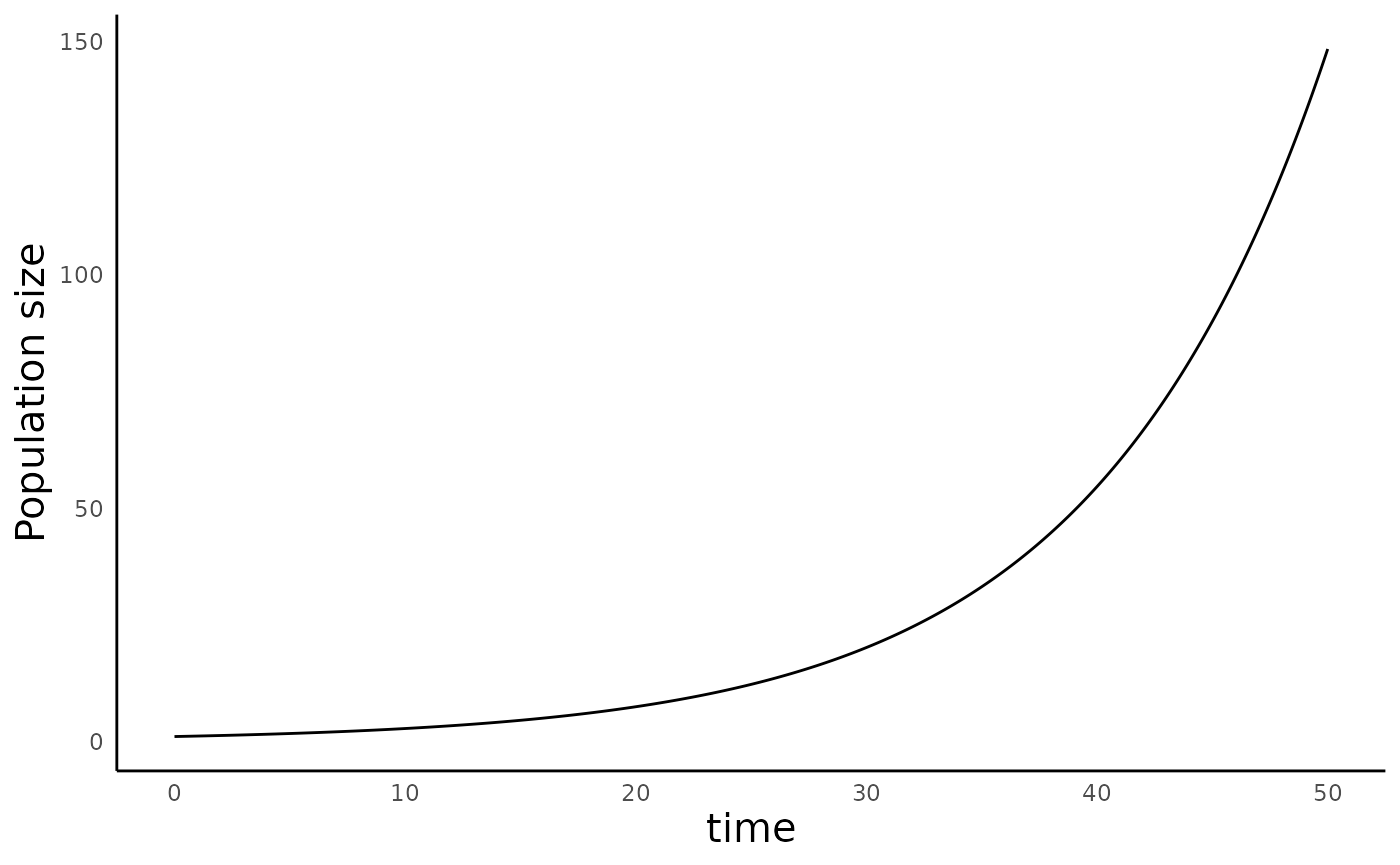

Logistic growth

The exponential growth model above is very straightforward, and predicts that in the long-term, any population experiencing such growth will reach an infinitely large size. Given that populations never grow without limits in nature, we can improve on this model.

Let us re-examine the assumptions of the exponential growth model– namely, that there is a per-capita birth rate \(b\) and a per-capita death rate \(d\) that stays constant at all times. We can simply relax this assumption by examining what happens when the net growth rate (\(rD\)) declines linearly as a population reaches an environmentally-determined carrying capacity (\(K\)). The dynamics of such a population can be described by the logistic growth equation:

\[\frac{dN}{dt} = rN \left(1-\frac{N}{K}\right)\]

Populations experience logistic growth can grow (i.e., have a positive population growth rate) until the population size is equal to the carrying capacity (\(N = K\)). When a population exceeds its carrying capacity, the population will have a negative growth rate, and shrink back to the carrying capacity. For more on this model, refer to this link.

We can simulate the dynamics of a population with logistic growth using the function run_logistic_model() as follows:

time_log <- seq(0, 100, 0.1) # length of time for model simulation
init_log <- c(N1 = 1) # initial population size 
params_log <- c(r = 0.2, K = 100) # population growth rate
sim_df_log <- run_logistic_model(time = time_log, init = init_log, params = params_log)

As above, this creates a data frame with columns for time and population size:

head(sim_df_log)
#>      time       N1
#> [1,]  0.0 1.000000
#> [2,]  0.1 1.019996
#> [3,]  0.2 1.040387
#> [4,]  0.3 1.061182
#> [5,]  0.4 1.082387
#> [6,]  0.5 1.104012

We can plot the trajectory of this population over time using the same code above:

plot_continuous_population_growth(sim_df_log)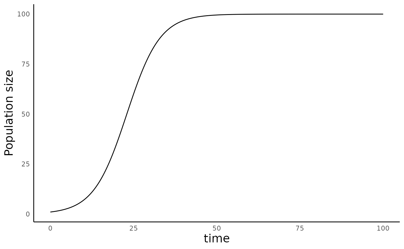

Lagged logistic growth

In some circumstances, the growth rate of a population might depend on the population size at some time in the past. For example, the reproductive output of individuals may be limited by how much they had to compete for resources as juveniles. We can model such a scenario by making the population growth rate at time \(t\) a function of some time \(t-\tau\) in the past as follows:

\[ \frac{dN}{dt} = rN_{t} \left(1-\frac{N_{t-\tau}}{K}\right)\]

We can model the dynamics of a population with lagged logistic growth using the same run_logistic_model() function as above, but we now simply need to define the additional parameter tau in the parameters vector:

time_laglog <- seq(0, 100, 0.1) # length of time for model simulation
init_laglog <- c(N1 = 1) # initial population size 
params_laglog <- c(r = 0.5, K = 100, tau = 2) # population growth rate
sim_df_laglog <- run_logistic_model(time = time_laglog, init = init_laglog, params = params_laglog)

This again produces a data frame with columns time and N1, though we are not showing it here to avoid repetition. At sufficiently large values of \(r\) and/or \(\tau\), this model results in damped oscillations in population sizes, before the population ultimately converges to its carrying capacity:

plot_continuous_population_growth(sim_df_laglog)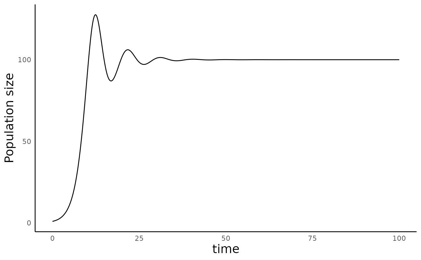

Discrete time models of population growth

The models above apply well to populations where births and deaths happen continuously, but they are not very relevant to species where births and deaths happen at discrete times (e.g. during a single breeding season). To model such species, we can turn to models of population growth in discrete time.

Exponential growth in discrete time

The simplest model of population growth in discrete time assumes that the population size at time \(t+1\) (\(N_{t+1}\)) is a product of the population size at time \(t\) (\(N_t\)) and the population growth rate, symbolized \(\lambda\):

\(N_{t+1} = \lambda N_t\)

When \(\lambda > 1\), the population grows every year, resulting in exponential growth, and when \(\lambda < 1\), the population shrinks to extinction. We can simulate the dynamics of such a population with the function run_discrete_exponential_model():

# We simply provide initial population size, lambda, and the time
# for simulation to the model as arguments:
sim_df_dexp <- run_discrete_exponential_model(N0 = 1, lambda = 1.2, time = 20)

This produces a data frame with columns time and N1:

head(sim_df_dexp)
#>   time      Nt
#> 1    0 1.00000
#> 2    1 1.20000
#> 3    2 1.44000
#> 4    3 1.72800
#> 5    4 2.07360
#> 6    5 2.48832

We can plot the population growth over time using the function plot_discrete_population_growth():

plot_discrete_population_growth(sim_df_dexp)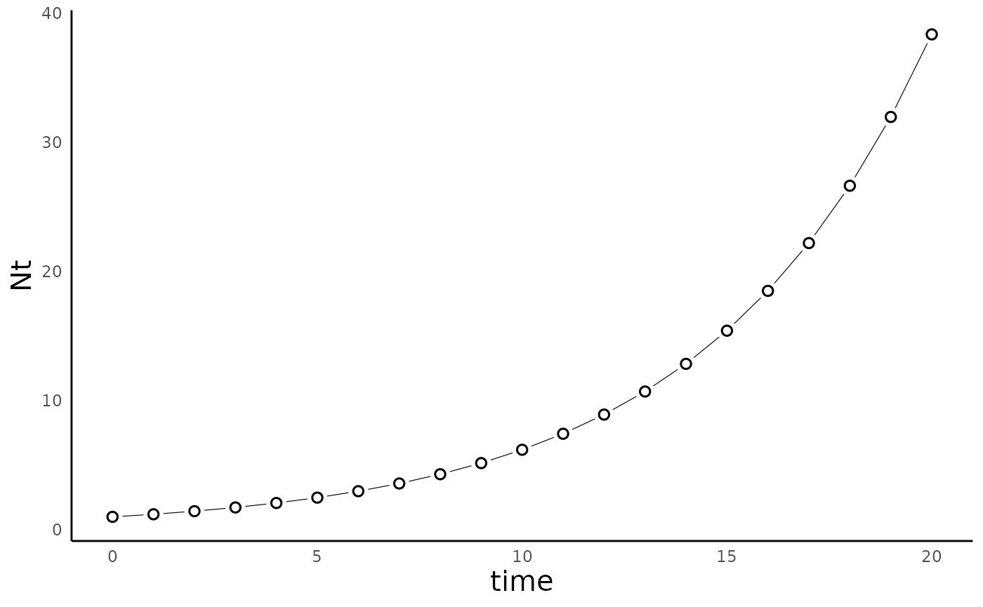

Logistic growth in discrete time

There are several ways we can build in limits to population growth in discrete time models. One of the most ‘obvious’ ways might be to convert the continuous time logistic growth model we met above into a model of discrete time population growth:

\[N_{t+1} = r_dN_t\left(1-\frac{N_t}{K}\right)\]

In this case, \(r_d\) takes the place of \(\lambda\), because it is the discrete version of the \(r\) parameter in the logistic growth model. Even though this seems like a fairly inocuous switch from continuous to discrete time, it turns out that this model is more interesting than it might look at first sight. In fact, this formulation was notably studied by Robert May in the classic 1976 paper “Simple mathematical models with very complicated dynamics”, in which he showed the potential for this model to generate chaotic dynamics. Another interesting aspect of this model is that unlike in the contiuous time model, \(K\) here doesn’t represent “carrying capacity” in the traditional sense, since the population doesn’t actually equilibrate to that population size – it equilibrates to a population size lower than \(K\). For more on this model, refer to this link.

We can simulate the model using the function run_discrete_logistic_model(), as follows:

params_disclog <- c(rd = 1.5, K = 1000)

sim_df_disclog <- run_discrete_logistic_model(N0 = 1, params = params_disclog, time = 50)

As above we can use the plot_discrete_population_growth() function to plot the dynamics of this model:

plot_discrete_population_growth(sim_df_disclog)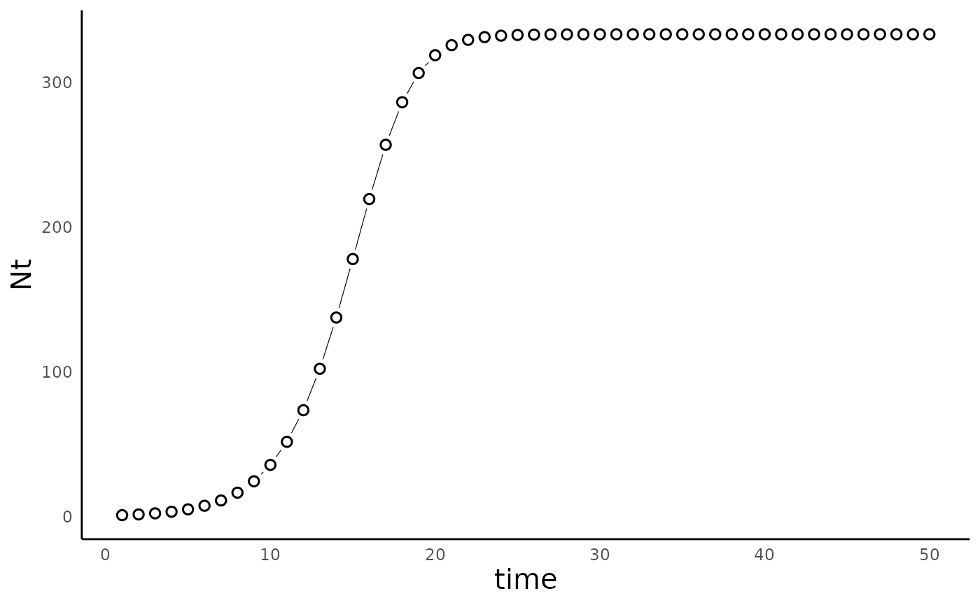

Robert May’s 1974 paper (show above) showed that at sufficiently large values of $r_d$, this simple model was capable of producing not only cyclic population dynamics, but also chaotic dynamics:

# By default, the run_discrete_logistic_model uses N0 = 1, so we can omit it here:
params_disclog_cyc = c(rd = 3, K = 1000)
sim_df_disclog_cyc <- run_discrete_logistic_model(params = params_disclog_cyc, time = 75)

params_disclog_chaos <- c(rd = 3.75, K = 1000)

sim_df_disclog_chaos <- run_discrete_logistic_model(params = params_disclog_chaos, time = 75)

plot_discrete_population_growth(sim_df_disclog_cyc) +
  plot_discrete_population_growth(sim_df_disclog_chaos)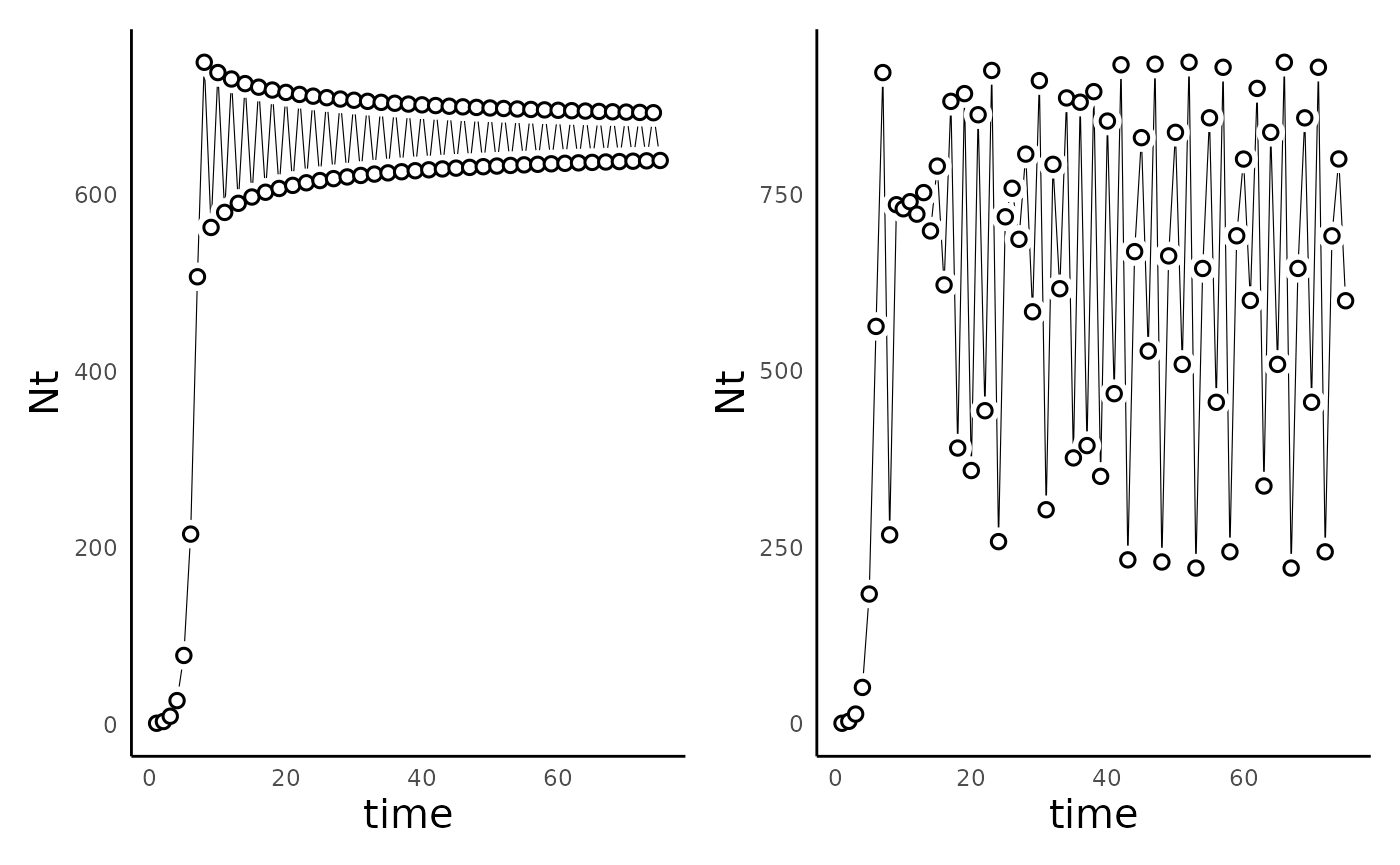

One helpful way to visualize the dynamics of a discrete logistic model is with a “cobweb plot”, which shows how the population at time \(t\) relates to the population at \(t+1\). For more information on cobweb plots, how to read them, and what they tell us, here are some useful references: link 1; link 2; link 3.

We can make a cobweb plot using the function plot_discrete_population_cobweb(). For this function, we need to provide the simulated data frame, as well as the parameter vector and the model type:

plot_discrete_population_cobweb(sim_df_disclog_cyc,
                                params_vec = params_disclog_cyc,
                                model_type = "discrete_logistic")
#> Warning: Removed 1 rows containing missing values (geom_segment).
#> Removed 1 rows containing missing values (geom_segment).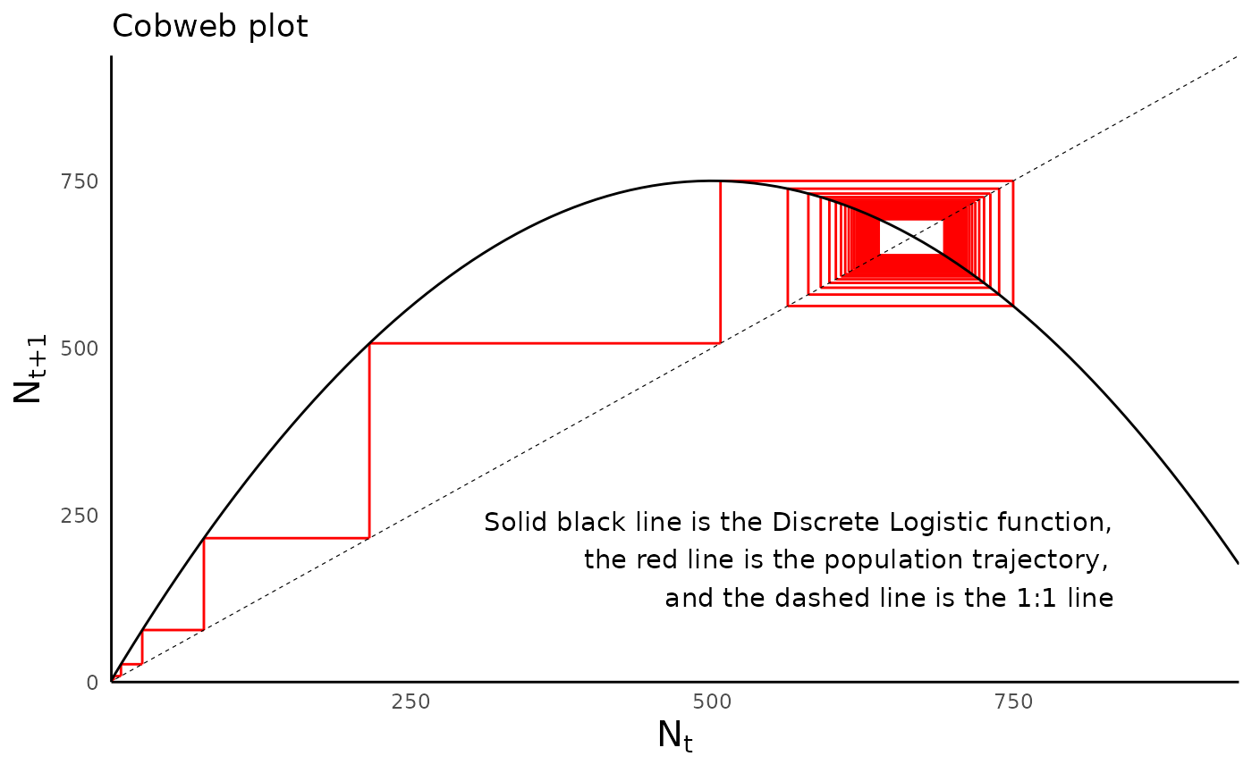

Compare the cobweb plot of the population with cyclic dynamics with that of the population with chaotic behavior:

plot_discrete_population_cobweb(sim_df_disclog_chaos,
                                params_vec = params_disclog_chaos,
                                model_type = "discrete_logistic")
#> Warning: Removed 1 rows containing missing values (geom_segment).
#> Removed 1 rows containing missing values (geom_segment).
#> Warning: Removed 15 row(s) containing missing values (geom_path).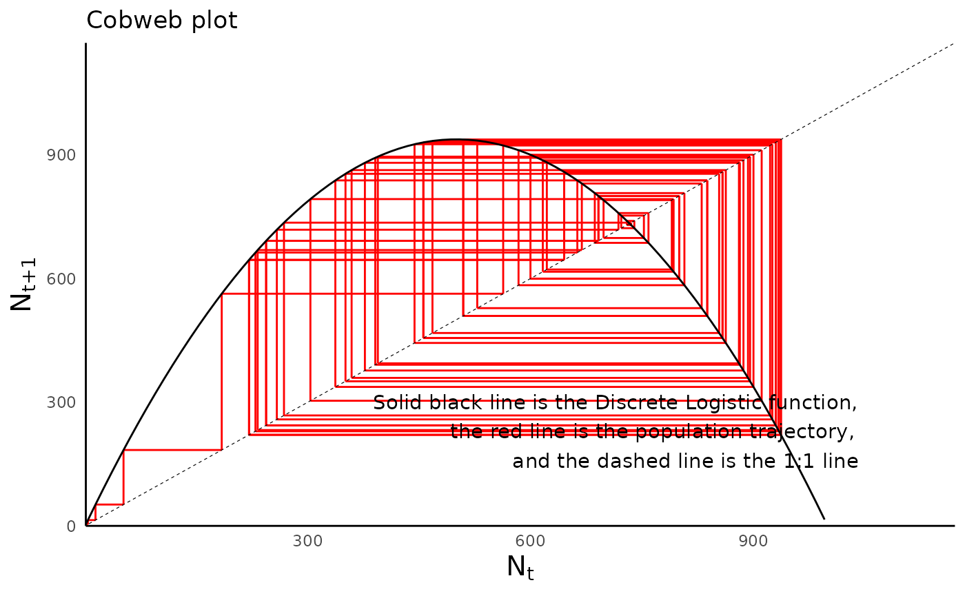

Other models of logistic growth in discrete time

As suggested above, there are several other commonly used models of population growth in discrete time, each with distinct behaviors and assumptions. Two models that are supported in ecoevoapps are the Beverton Holt model and the Ricker model. Both of these were developed in the context of fisheries management but have since been applied to various other organisms.

Beverton Holt model

The Beverton-Holt model models population dynamics as follows:

\[N_{t+1} = \frac{RN_t}{1+\left(\frac{R-1}{K}\right)N_t}\]

Ricker model

The Ricker model models population dynamics as follows: \[N_{t+1} = N_t e^{(r (1 - N_t/K))}\]

Simulating in ecoevoapps

The Beverton-Holt model and Ricker model can be simulated in ecoevoapps using the functions run_beverton_holt_model() and run_ricker_model() respectively. The usage is same as in the discrete logistic model above, so we won’t repeat the code here for brevity. To make cobweb plots, note that the parameter model_type in plot_discrete_population_cobweb needs to be set to beverton_holt or ricker as appropriate.

Structured population growth

The models above assume that within populations, all individuals have equal rates of reproduction and death. But in fact, some populations are best modeled as a collection of individuals in distinct age classes (Tenhumberg, 2010). The growth of such structured populations depends on the transition rates from one age class to another. For example, the survival rates of juveniles into young adults may be different from the survival rate of young adults into older adults. We can model the dynamics of such populations by knowing the rates of survival from one age class into the next, and by knowing how individuals in each age contribute to the population by giving birth to new individuals.

The Leslie matrix

The Leslie Matrix is a convenient way of organizing age transition rates (survival and fecundity). The Leslie matrix is an \(NxN\) matrix, where \(N\) indicates the total number of ages in the population cycle. The elements of the matrix tell us about how the individuals in each age column contribute to each age row. For example, the second column in the first row tells us how individuals who are of age 2 contribute to the age 1 category.

In addition to being a convenient way to account for survival and fecundity information, the matrix also has three key properties:

1. To simulate the population at the next time step (time \(t+1\)), one simply needs to multiply the Leslie matrix by the matrix with the initial population sizes (at time \(t\)).

2. The largest eigenvalue of the Leslie matrix is \(\lambda\), the asymptotic growth rate for the whole population. When \(\lambda < 1\) the declines to extinction, \(\lambda > 1\) the grows exponentially, and when \(\lambda = 1\) the population size remains constant through time).

3. The eigenvector that corresponds to the largest eigenvalue gives the stable population structure, i.e., the proportions of each age class after the population reached equilibrium.

Simulating structured population dynamics in R

We can model the dynamics of an age-structured population using the function run_structured_population_simulation() as follows:

# define the Leslie matrix:
leslie_mat <- matrix(c(0, 8, 1, 1, 
                      0.4, 0, 0, 0, 
                      0, 0.8, 0, 0, 
                      0, 0, 0.1, 0), 
                    ncol = 4, byrow = T)
# define a vector of initial population sizes in each class:
init_vec <- c(10, 0, 0, 0)

structured_popgrowth <- run_structured_population_simulation(leslie_mat = leslie_mat, init = init_vec, time = 50)

Before we visualize the model output, we can make a population structure diagram for the defined Leslie matrix using the function plot_leslie_diagram():

plot_leslie_diagram(leslie_mat)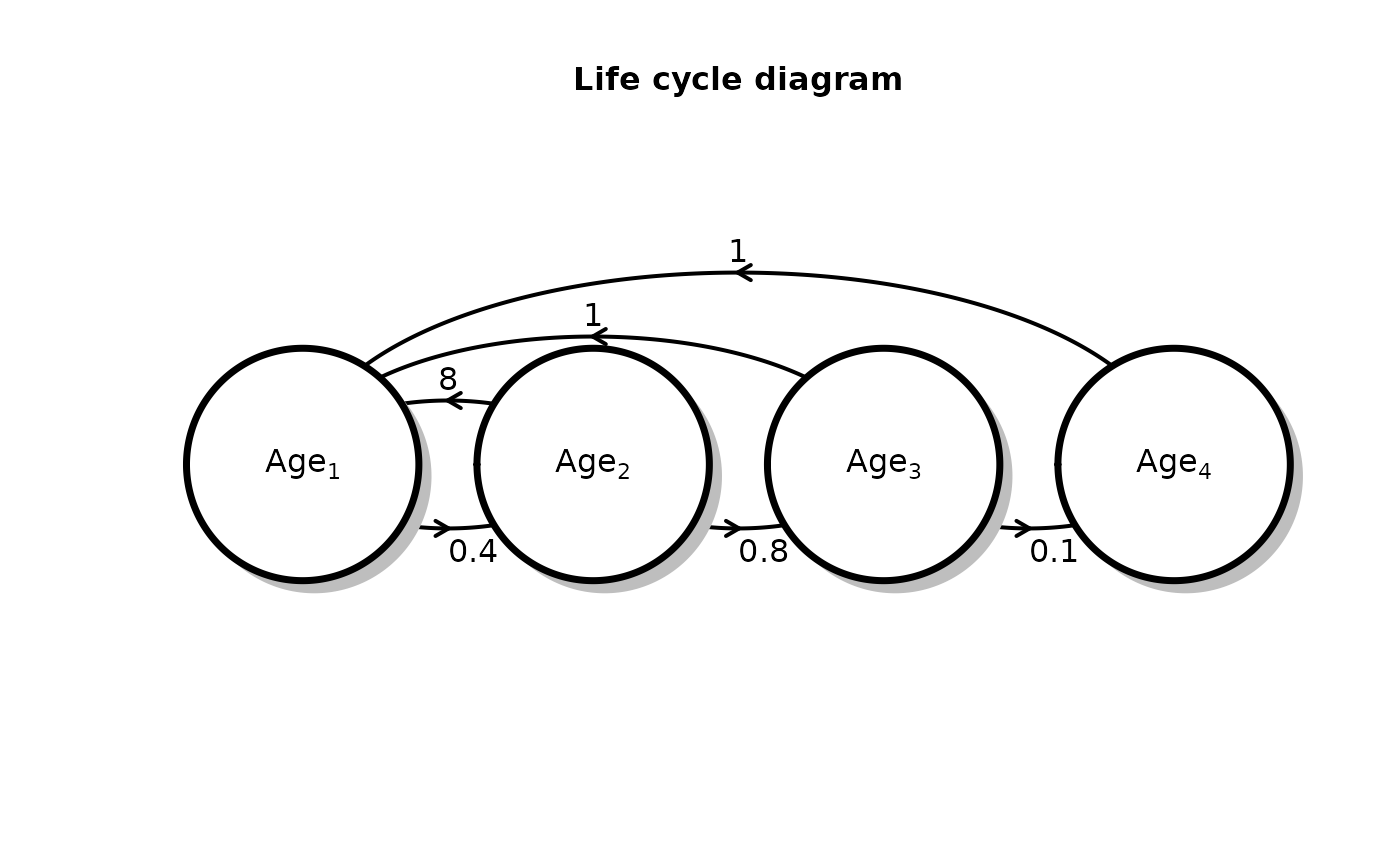

#> $arr
#>   row col Angle Value   rad    ArrowX    ArrowY TextX TextY
#> 1   2   1     0   0.4 0.125 0.2494110 0.2750014 0.250 0.255
#> 2   1   2     0     8 0.125 0.2501963 0.5249998 0.250 0.545
#> 3   3   2     0   0.8 0.125 0.4994110 0.2750014 0.500 0.255
#> 4   1   3     0     1 0.250 0.3753927 0.6499997 0.375 0.670
#> 5   4   3     0   0.1 0.125 0.7494110 0.2750014 0.750 0.255
#> 6   1   4     0     1 0.375 0.5005890 0.7749995 0.500 0.795
#> 
#> $comp
#>          x   y
#> [1,] 0.125 0.4
#> [2,] 0.375 0.4
#> [3,] 0.625 0.4
#> [4,] 0.875 0.4
#> 
#> $radii
#>        x         y
#> [1,] 0.1 0.2270617
#> [2,] 0.1 0.2270617
#> [3,] 0.1 0.2270617
#> [4,] 0.1 0.2270617
#> 
#> $rect
#>      xleft      ybot xright      ytop
#> [1,] 0.025 0.1729383  0.225 0.6270617
#> [2,] 0.275 0.1729383  0.475 0.6270617
#> [3,] 0.525 0.1729383  0.725 0.6270617
#> [4,] 0.775 0.1729383  0.975 0.6270617

This function generates a matrix with as many rows as the number of age classes defined in the leslie matrix, and as many columns as the number of time steps (plus the initial time step):

dim(structured_popgrowth)
#> [1]  4 51

We can plot the number of individuals in each age class using the function plot_structured_population_agedist() :

plot_structured_population_size(structured_popgrowth)
#> Warning: Transformation introduced infinite values in continuous y-axis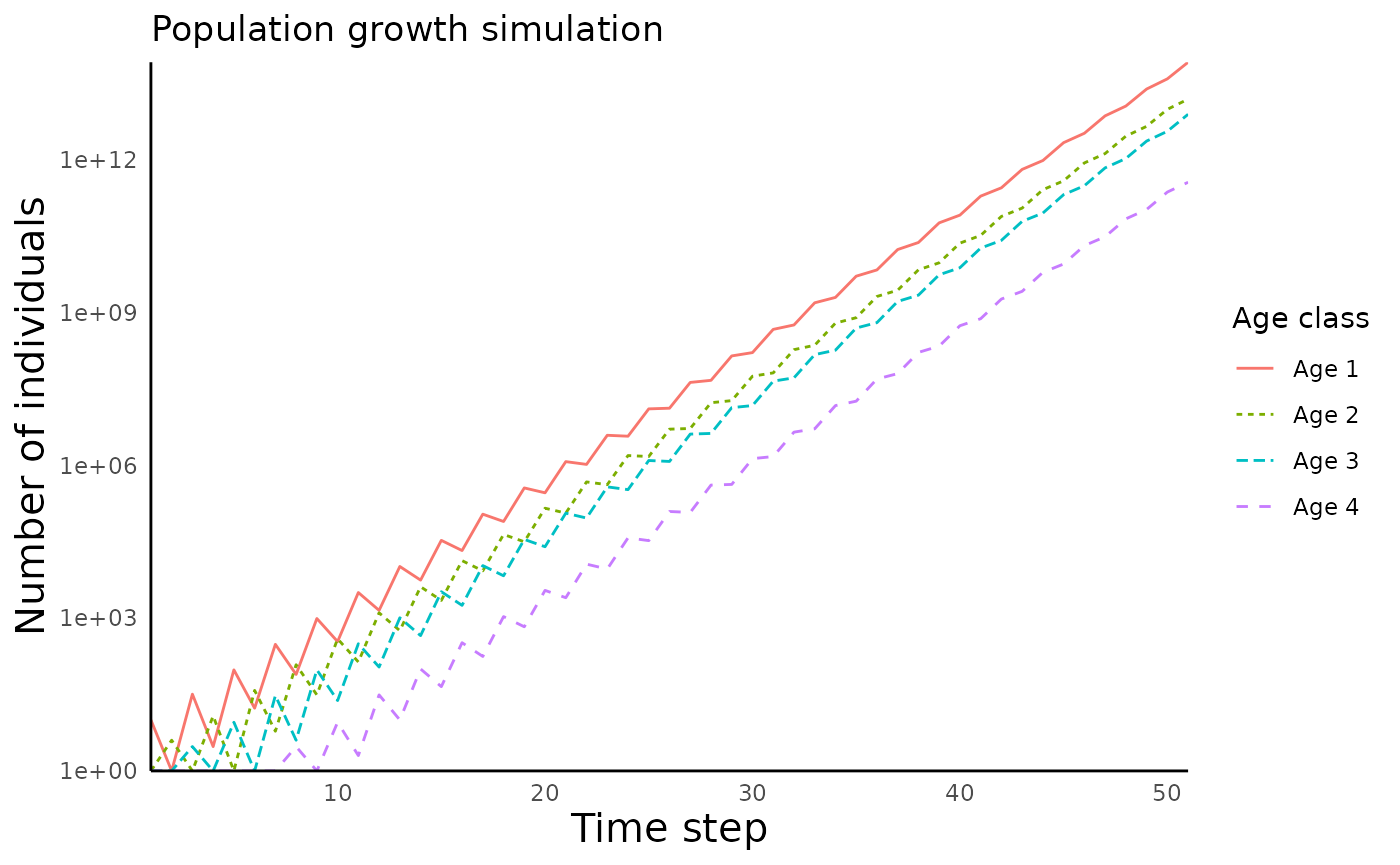

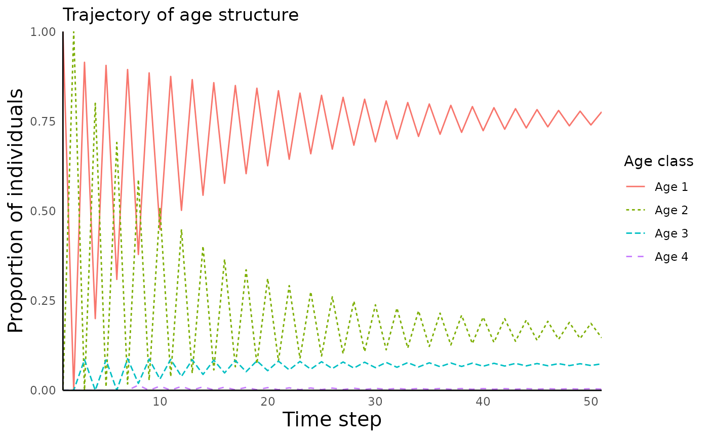
We can also plot the proportion of individuals in each age class using the function plot_structured_population_agedist():

plot_structured_population_agedist(structured_popgrowth)