Infectious disease dynamics (compartment/SIR models)
sir-dynamics.RmdThere is an important category of models from epidemiology called Compartment models. These models are designed to model the spread of diseases through populations that are made of individuals in different compartments (groups). For example, a population might be made up of individuals who are susceptible to the disease, individuals who have been exposed to a disease but are not yet infected/infectious, infected individuals who can spread disease, recovered individuals, etc. Different models can include different compartments, based on the population being studied and the dynamics of the infection. For more details on compartment models, please refer to the Wikipedia page or refer to this paper.
The ecoevoapps package includes functions to simulate
various specific implementations of such compartment models.
Suscptible-Infectious-Recovered (SIR) model
One of the most common implementations of compartment models tracks the dynamics of a population comprised of individuals who are susceptible to a disease, those who are infectious, and those who have recovered. The dynamics of a such a model are governed by the following set of equations:
\[ \begin{align} \frac{dS}{dt} &= m(S + I + R)(1 - v) - mS - \beta SI\\ \frac{dI}{dt} &= \beta SI - mI - \gamma I\\ \frac{dR}{dt} &= \gamma I - mR + mv(S + I + R) \end{align} \]
This model can be simulated with the
run_infectiousdisease_model() function:
sir_params_vec <- c(m = .1, beta = .01, v = .2, gamma = 0)
sir_init_vec <- c(S = 100, I = 1, R = 0)
sir_time_vec <- seq(0, 25, 0.1)
sir_out <- run_infectiousdisease_model(time = sir_time_vec, init = sir_init_vec, params = sir_params_vec, model_type = "SIR")
head(sir_out)
#>   time         S        I         R
#> 1  0.0 100.00000 1.000000 0.0000000
#> 2  0.1  99.70499 1.094015 0.2009934
#> 3  0.2  99.40350 1.196509 0.3999868
#> 4  0.3  99.09479 1.308208 0.5970002
#> 5  0.4  98.77806 1.429887 0.7920533
#> 6  0.5  98.45245 1.562382 0.9851656
We can then use plot_infectiousdisease_time() to plot
the trajectory of these compartments over time:
plot_infectiousdisease_time(sir_out, model_type = "SIR")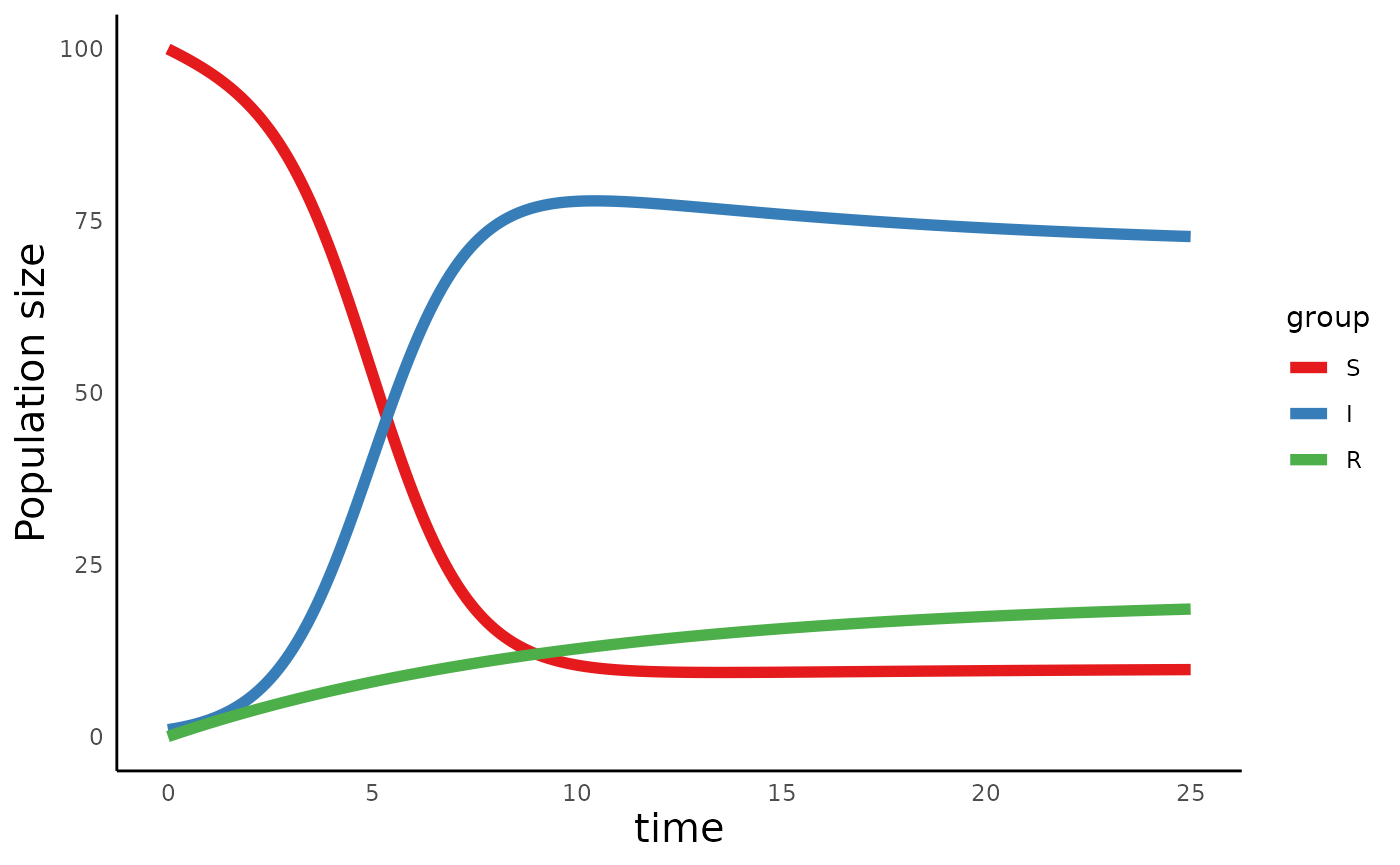
We can also use plot_infectiousdisease_portrait() to
track how the compartments change relative to one another:
plot_infectiousdisease_portrait(sir_out, "S", "I") +
  plot_infectiousdisease_portrait(sir_out, "S", "R") +
  plot_infectiousdisease_portrait(sir_out, "R", "I")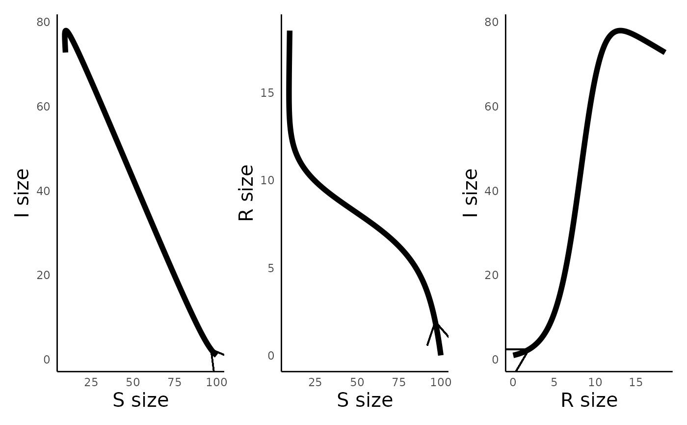
Susceptible-Infectious-Susceptible
In the SIR model, once an individual recovers from a disease, they are fully immune to it in the future. But in reality, we may encounter a disease from which individuals never actually develops immunity. In this case, an SIS model may be more appropriate:
\[ \begin{align} \frac{dS}{dt} &= m(S + I) - mS - \beta SI + \gamma I\\ \frac{dI}{dt} &= \beta SI - mI - \gamma I\\ \end{align} \]
We can similarly simulate the dynamics of an SIS model using the same functions as above, just with different inputs:
sis_params_vec <- c(m = 0.1, beta = .01, gamma = 0)
sis_init_vec <- c(S = 100, I = 1)
sis_time_vec <- seq(0, 25, 0.1)
sis_out <- run_infectiousdisease_model(time = sis_time_vec, init = sis_init_vec, params = sis_params_vec, model_type = "SIS")
head(sis_out)
#>   time         S        I
#> 1  0.0 100.00000 1.000000
#> 2  0.1  99.90588 1.094125
#> 3  0.2  99.80301 1.196989
#> 4  0.3  99.69062 1.309385
#> 5  0.4  99.56783 1.432166
#> 6  0.5  99.43374 1.566258

plot_infectiousdisease_time(sis_out, model_type = "SIS")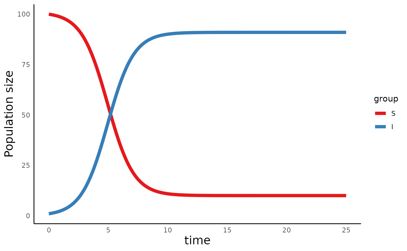
Susceptible-Exposed-Infectious-Recovered
Another structure we can explore is cases in which populations are comprised of susceptible individuals, those who are exposed but not (yet) infectious, infectious individuals, and those who have recovered. This is captured by an SEIR model:
\[ \begin{align} \frac{dS}{dt} &= m(S + E + I + R)(1 - v) - mS - \beta SI\\ \frac{dE}{dt} &= \beta SI - aE - mE\\ \frac{dI}{dt} &= aE - mI - \gamma I\\ \frac{dR}{dt} &= \gamma I - mR + mv(S + E + I + R) \end{align} \]
Again, we can use the functions above with different input parameters to simulate this model:
seir_params_vec <- c(m = 0.1, beta = .1, gamma = 0.2, a = .025, v = 0)
seir_init_vec <- c(S = 100, E = 0, I = 2, R = 0)
seir_time_vec <- seq(0, 25, 0.1)
seir_out <- run_infectiousdisease_model(time = seir_time_vec, init = seir_init_vec, params = seir_params_vec, model_type = "SEIR")
head(seir_out)
#>   time         S        E        I          R
#> 1  0.0 100.00000 0.000000 2.000000 0.00000000
#> 2  0.1  98.07764 1.939821 1.943316 0.03922482
#> 3  0.2  96.26275 3.767312 1.892944 0.07699503
#> 4  0.3  94.54461 5.493511 1.848433 0.11344615
#> 5  0.4  92.91365 7.128267 1.809374 0.14870377
#> 6  0.5  91.36133 8.680395 1.775392 0.18288448

plot_infectiousdisease_time(seir_out, model_type = "SEIR")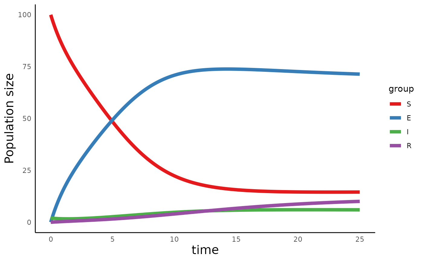
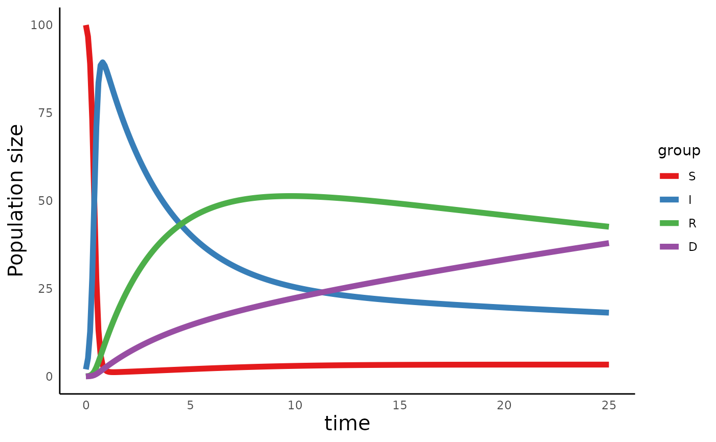
Susceptible-Infectious-Recovered-Dead
In all the models above, we assume that individuals who are infected can eventually recover, and that there is no excess mortality associated with the disease. But we know that in some cases, disease condition is associated with increased mortality rates, which we can model by introducing a new compartment into these models:
\[ \begin{align} \frac{dS}{dt} &= m(S + I + R)(1 - v) - mS - \beta SI\\ \frac{dI}{dt} &= \beta SI - mI - \gamma I - \mu I\\ \frac{dR}{dt} &= \gamma I - mR + mv(S + I + R)\\ \frac{dD}{dt} &= \mu I\\ \end{align} \]
We can simulate this model as follows:
sird_params_vec <- c(m = 0.1, beta = .1, gamma = 0.2, a = .025, v = 0, mu = 0.05)
sird_init_vec <- c(S = 100, I = 2, R = 0, D = 0)
sird_time_vec <- seq(0, 25, 0.1)
sird_out <- run_infectiousdisease_model(time = sird_time_vec, init = sird_init_vec, params = sird_params_vec, model_type = "SIRD")
head(sird_out)
#>   time         S         I          R          D
#> 1  0.0 100.00000  2.000000 0.00000000 0.00000000
#> 2  0.1  96.73916  5.177384 0.06670921 0.01674776
#> 3  0.2  88.98754 12.719265 0.23422390 0.05897178
#> 4  0.3  73.35545 27.866251 0.62150467 0.15679934
#> 5  0.4  50.17209 50.093202 1.38469627 0.35001329
#> 6  0.5  27.70540 71.051871 2.58721061 0.65552138

plot_infectiousdisease_time(sird_out, model_type = "SIRD")