Mechanistic models of competition for biotic/abiotic resources • ecoevoapps

library(ecoevoapps)

This vignette illustrates how ecoevoapps can be used to simulate two different models of explicit resource competition between species. In the first model, two consumer species compete for a shared biotic prey, while in the second model, two consumers compete for two shared abiotic resources.

Competition for a biotic resource

In this model, two consumer species (\(P_1\) and \(P_2\)) require the same resource species (\(H\)) to grow. An increase in \(P_1\) results in a decreased growth rate of \(P_2\) because of \(P_1\)’s suppression of resource \(H\). Thus, while the model doesn’t include any explicit competition between the two consumers, these two species nevertheless do compete with one another for the shared resource.

Even this fairly straightforward scenario can be modeled in many ways. E.g. we can consider a resource species \(H\) that, in the absence of either consumer, grows either exponentially (with no intrinsic limit to population growth), or logistically.

The models can also consider different relationships between the density of resources and rate at which they are attacked by consumers. This relationship is called the functional response, and we consider two types of relationships. First, we consider a “Type 1 functional response”, in which the rate at which consumers consume resources is a linear function of the resource density. The second relationship is the “Type II functional response”, in which the amount of resources consumed is a saturating function of resource density. The idea of the Type II functional response was developed by C.S. Holling in the 1959 paper “Some characteristics of simple types of predation and parasitism”.

This system of equations describes the most complex version of this model:

\[ \begin{align} \frac{dH}{dt} &= rH \bigl(1-qH\bigr) - \frac{a_1HP_1}{1+a_1T_{h1}H} - \frac{a_2HP_2}{1+a_2T_{h2}H} \\ \\ \frac{dP_1}{dt} &= e_{1} \frac{a_1HP_1}{1+a_1T_{h1}H} - d_1P_1 \\ \\ \frac{dP2}{dt} &= e_2 \frac{a_2HP_2}{1+a_2T_{h2}H} - d_2P_2 \end{align} \]

We can simulate this model using ecoevoapps::run_biotic_comp_model():


bioticRC_time = seq(0,250,0.1)
bioticRC_init = c(H = 30, P1 = 25, P2 = 25)
bioticRC_params = c(r = 0.2, q = .0066, 
                    a1 = .02, T_h1 = 0.1, e1 = 0.4, d1 = 0.1, 
                    a2 = .02, T_h2 = 0.1, e2 = 0.39, d2 = 0.1)

bioticRC_simulation <- run_biotic_comp_model(time = bioticRC_time, init = bioticRC_init, params = bioticRC_params)

This generates a dataframe with columns time, P1, P1, and H:

head(bioticRC_simulation, 5)
#>      time        H       P1       P2
#> [1,]  0.0 30.00000 25.00000 25.00000
#> [2,]  0.1 27.72356 25.29726 25.28347
#> [3,]  0.2 25.59066 25.55758 25.53072
#> [4,]  0.3 23.59810 25.78204 25.74288
#> [5,]  0.4 21.74164 25.97200 25.92131

We can then use the ecoevoapps function plot_biotic_comp_time() to generate a trajectory of these populations over time:

plot_biotic_comp_time(bioticRC_simulation)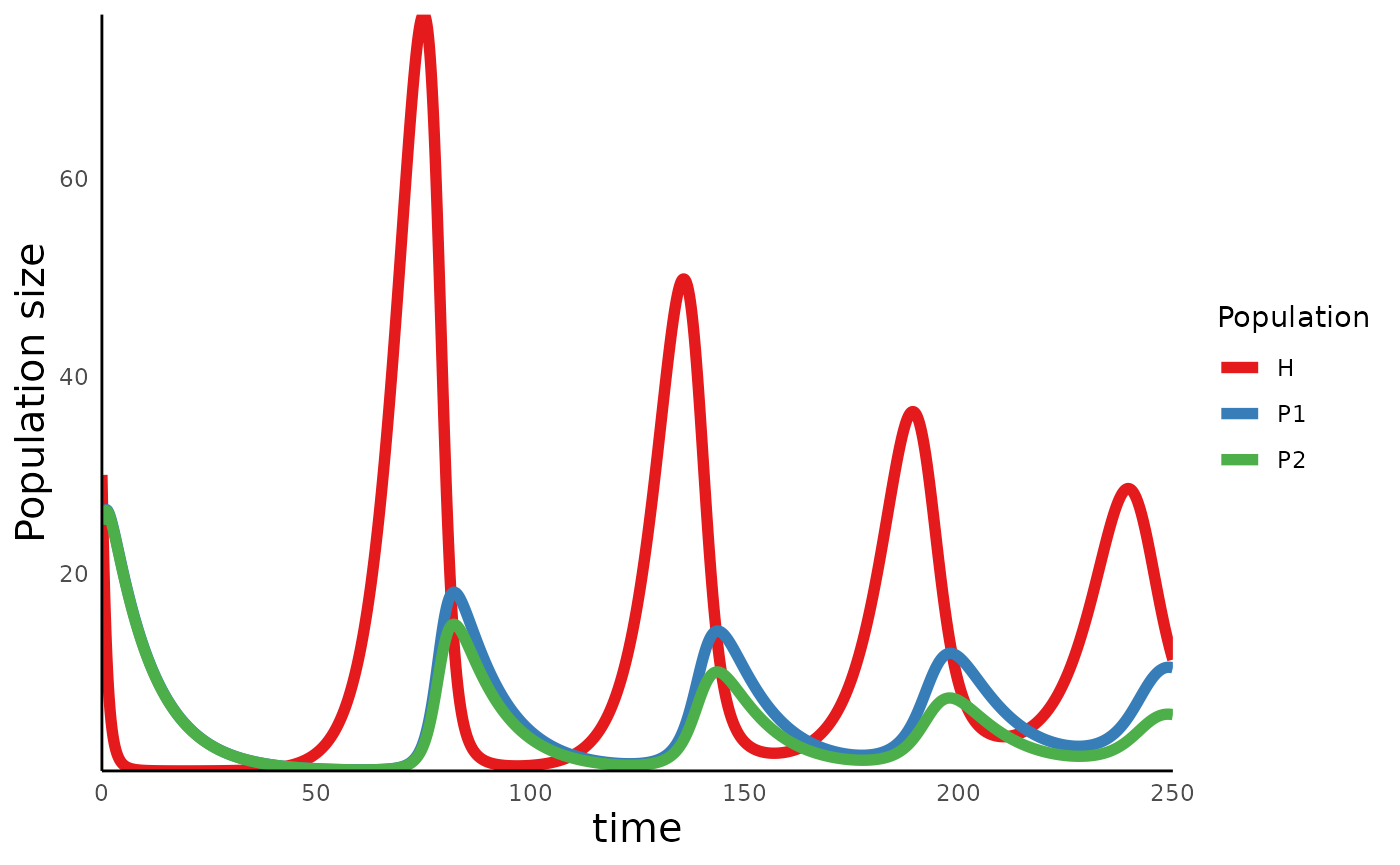

Competition for abiotic resources

In the model above, the resource \(H\) represent biotic resources that follow the rules of exponential or logistic single population growth. But in other cases, species may compete for abiotic resources (e.g. nutrients) whose dynamics aren’t captured by standard population dynamics models.

One suite of models that captures such dynamics is the resource competition models developed by Dave Tilman in a series of papers in the 1980s. ecoevoapps implements one particular version of these models, in which two species compete for two resources, which are both essential for their growth. The dynamics of consumers and the resource species are described by the following equations:

Resource dynamics equations

\[\frac{dR_1}{dt} = a_1(S_1-R_1) - N_1c_{11}\left(\frac{1}{N_1}\frac{dN_1}{dt} + m_1\right) - N_2c_{21}\left(\frac{1}{N_2}\frac{dN_2}{dt} + m_2\right)\] \[\frac{dR_2}{dt} = a_2(S_2-R_2) - N_2c_{12}\left(\frac{1}{N_1}\frac{dN_1}{dt} + m_1\right) - N_2c_{22}\left(\frac{1}{N_2}\frac{dN_2}{dt} + m_2\right)\]

Consumer dynamics equations

\[\frac{1}{N_1}\frac{dN_1}{dt} = \mathrm{min}\left(\frac{r_1R_1}{R_1 + k_{11}} - m_1 ,\frac{r_2R_2}{R_2 + k_{12}} - m_1\right)\]

\[\frac{1}{N_2}\frac{dN_2}{dt} = \mathrm{min}\left(\frac{r_1R_1}{R_1 + k_{21}} - m_2 ,\frac{r_2R_2}{R_2 + k_{22}} - m_2\right)\]

In the consumer dynamics equation above, the rate of growth for both species is determined by whichever resource is more limiting (which is implemented by the use of the min function in the equations). The key insight from Tilman’s work was that two species can coexist when each species is the strongest competitor (i.e. can tolerate the lowest minimum amount) for different resources (see the R-star rule).

This model can be implemented in ecoevoapps using the function

abiotic_rc_time <- seq(0,50,0.1)
abiotic_rc_init <- c(N1 = 10, N2 = 10, R1 = 20, R2 = 20)
abiotic_rc_params <- c(S1 = 12, S2 = 12, r1 = 1.6, r2 = 1, k11 = 18, k12 = 4,
                       k21 = 2, k22 = 14, m1 = .2, m2 = .2,c11 = .25, c12 = .08, 
                       c21 = .1, c22 = .2, a1 = .5, a2 = .5)
sim_df_abiotic_rc <- run_abiotic_comp_model(time = abiotic_rc_time, init = abiotic_rc_init, params = abiotic_rc_params)
head(abiotic_rc_params, 5)
#>   S1   S2   r1   r2  k11 
#> 12.0 12.0  1.6  1.0 18.0

The trajectory of resources and consumers through time can be plotted with plot_abiotic_comp_time():

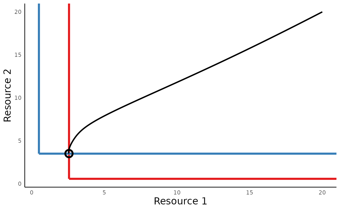
plot_abiotic_comp_time(sim_df_abiotic_rc)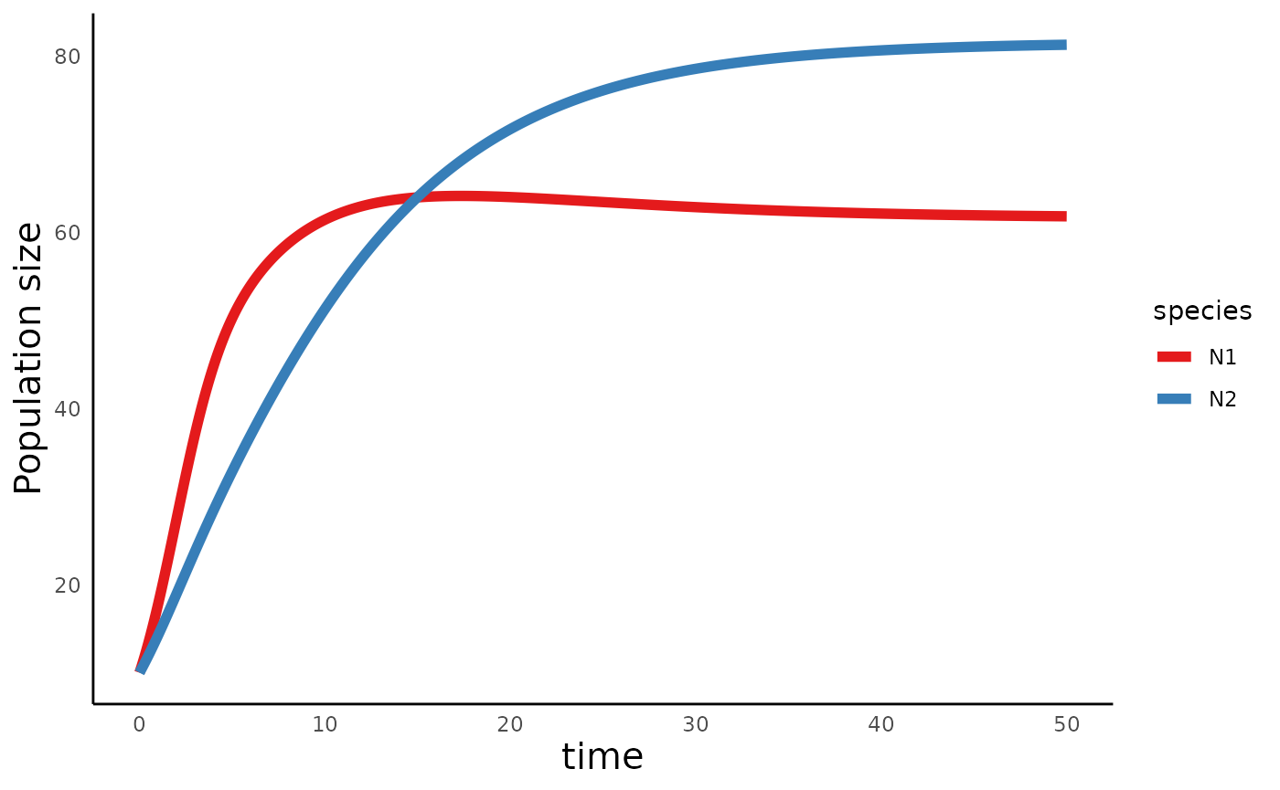

The package also includes functions to calculate the R* (run_abiotic_comp_rstar()) and to visualize the trajectory of resource levels (plot_abiotic_comp_portrait()):

rstar_vec <- run_abiotic_comp_rstar(params = abiotic_rc_params)
rstar_vec # Note that Rij us the R* for consumer i, resource j
#>       R11       R12       R21       R22 
#> 2.5714286 0.5714286 0.5000000 3.5000000
plot_abiotic_comp_portrait(rstar_vec = rstar_vec, sim_df = sim_df_abiotic_rc)