Differential equations in R • ecoevoapps

Behind the scenes, ecoevoapps uses the wonderful deSolve package to solve the differential equations in R. If you want to explore how this package works so that you can simulate the dynamics of your own favorite model or tweak existing models in ecoevoapps, read on!

To use deSolve, we first need to write a function that describes the differential equations, which we can then solve using the function deSolve::ode().

Example 1 - Lotka-Volterra competition

If we want to run the Lotka-Volterra competition model in R, we first write a function using the syntax as follows:

# Hand-coding the Lotka-Volterra competition model
lotka_volterra_competition <- function(time, init, params) {
  with (as.list(c(time, init, params)), {
    # description of parameters
    # r1 = per capita growth rate of species 1
    # N1 = population size of species 1
    # K1 = carying capacity of species 1
    # a = relative per capita effect of species 2 on species 1
    # r2 = per capita growth rate of species 2
    # N2 = population size of species 2
    # K2 = carrying capacity of species 2
    # b = relative per capita effect of species 1 on species 2

    # Differential equations
    dN1 <- r1*N1*(1 - (N1 + a*N2)/K1)
    dN2 <- r2*N2*(1 - (N2 + b*N1)/K2)

    # Return dN1 and dN2
    return(list(c(dN1, dN2)))
  })
}

With this function defined, we can now define the parameter values, initial values, and time over which we want to run a simulation:

# define vectors of initial population sizes, time, and parameters
# define initial population sizes for the two species
init <- c(N1 = 10, N2 = 30)
time <- seq(0,500, by = 0.1)
# define the parameter vector -- note that the names should match
# the parameter names we used in the lotka_volterra_competition function above
params <- c(r1 = .2, r2 = .1, K1 = 500, K2 = 600, a = .9, b = 1.1)

We are now ready to simulate the dynamics as follows:

lv_out <- deSolve::ode(func = lotka_volterra_competition,
                       y = init, times = time, parms = params)
# Plot model output
plot(lv_out[,"N1"]~lv_out[,"time"], type = "l", ylim = c(0, 700))
lines(lv_out[,"N2"]~lv_out[,"time"], type = "l", col = 2)

Example 2 - predator-prey dynamics

This example shows how the same approach can be used to simulate the Lotka-Volterra predator-prey model with logistic growth in the prey species:

# Define the function
lv_predprey_logPrey <- function(time,init,pars) {
  with (as.list(c(time,init,pars)), {
    # description of parameters:
    # r = per capita growth rate (prey)
    # a = attack rate
    # e = conversion efficiency
    # d = predator death rate
    # K = carrying capacity of the prey

    dH = r*H*(1 - H/K) - (a*H*P)
    dP = e*(a*H*P) - d*P
    return(list(c(dH = dH, dP = dP)))

  })
}

# Define parameters and initial conditions
time <- seq(0, 250, 0.1)
init <- c(H = 10, P = 10)
params <- c(r = 1, K = 250, a = 0.1, e = 0.2, d = 0.25)

# Now, we are ready to run the mode:

predprey_out <- deSolve::ode(func = lv_predprey_logPrey,
                       y = init, times = time, parms = params)
# Plot model output
plot(predprey_out[,"H"]~predprey_out[,"time"], type = "l", ylim = c(0,16))
lines(predprey_out[,"P"]~predprey_out[,"time"], type = "l", col = 2)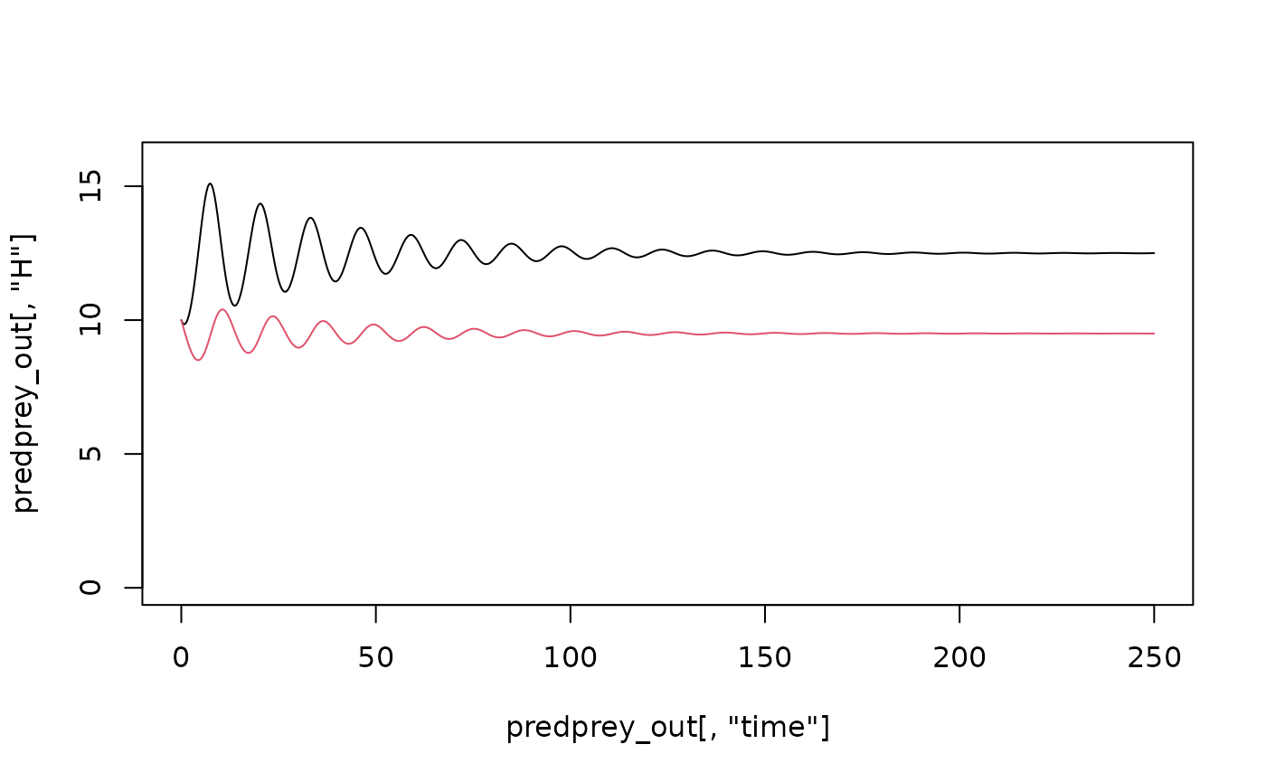

More resources

We also strongly recommend that you explore some deSolve tutorials to understand the workflow. (ex. 1; ex. 2; there’s also an example specifically on the Lotka-Volterra predator-prey models!). The package also includes the function deSolve::dede(), which we use in ecoevoapps to simulate the delayed-differential model for logistic growth (see run_logistic_model()).