Lotka-Volterra competition model
lotka-volterra-competition.RmdThe simplest model of interspecific competition included in this package is the two-species Lotka Volterra competition model. In this model, the population growth rate of each species is determined by the density of that species itself, as well as the density of its competitor species. For example, the growth rate of species \(1\) (\(\frac{dN_1}{dt}\)) is determined by the abundance of that species (\(N_1\)), the species’ carrying capacity (\(K_1\)), the density of species 2 (\(N_2\)), and by the relative competitive effect of species \(2\) on species \(1\)):
\[\frac{dN_1}{dt} = r_1N_1\big(1-\frac{N_1 + \alpha N_2}{K_1}\big)\] If the two species are close competitors, then \(\alpha \to 1\), such that the growth of species \(1\) is equally affected by the density of both species.
Similarly, the growth rate of species \(2\) is as follows: \[\frac{dN_2}{dt} = r_2N_2\big(1-\frac{N_2 + \beta N_1}{K_2}\big)\] where \(\beta\) now describes the relative competitive effect of species \(1\) on species \(2\).
We can simulate the dynamics of this model using
ecoevoapps using the function
run_lvcomp_model() as follows:
library(ecoevoapps)

lvcomp_time <- seq(0, 100, 0.1)
lvcomp_init <- c(N1 = 70, N2 = 50)
lvcomp_params <- c(r1 = .1, r2 = .15, K1 = 500, K2 = 600, a = .5, b = .5)
lvcomp_simulation <- run_lvcomp_model(time = lvcomp_time, init = lvcomp_init,
                                      params = lvcomp_params)
This generates a dataframe with columns time,
N1, and N2:
head(lvcomp_simulation)
#>      time       N1       N2
#> [1,]  0.0 70.00000 50.00000
#> [2,]  0.1 70.56867 50.64733
#> [3,]  0.2 71.14069 51.30183
#> [4,]  0.3 71.71605 51.96357
#> [5,]  0.4 72.29475 52.63258
#> [6,]  0.5 72.87678 53.30893
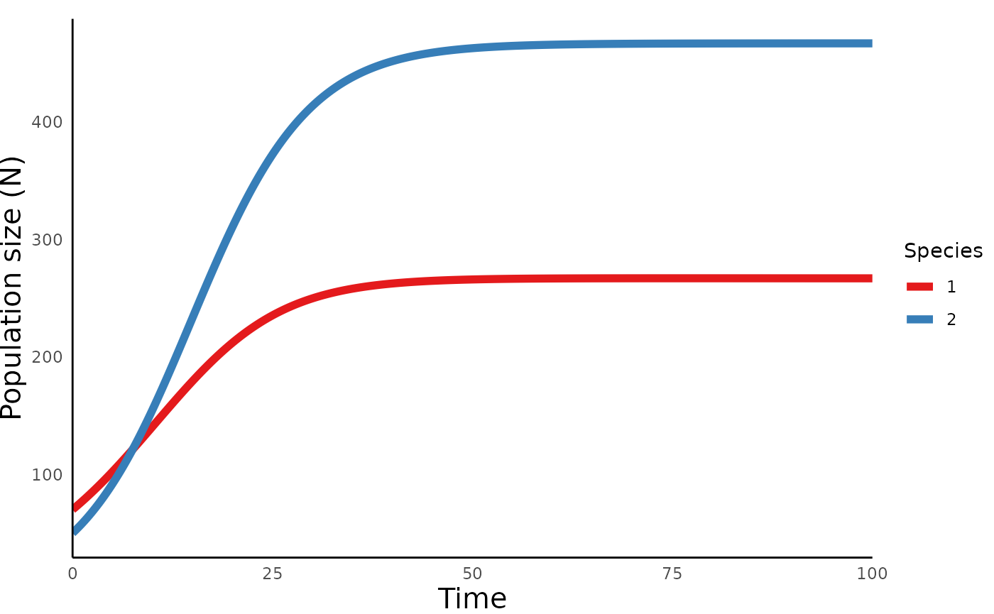
We can then use the ecoevoapps function
plot_lvcomp_time() to generate a trajectory of these
populations over time:
plot_lvcomp_time(lvcomp_simulation)
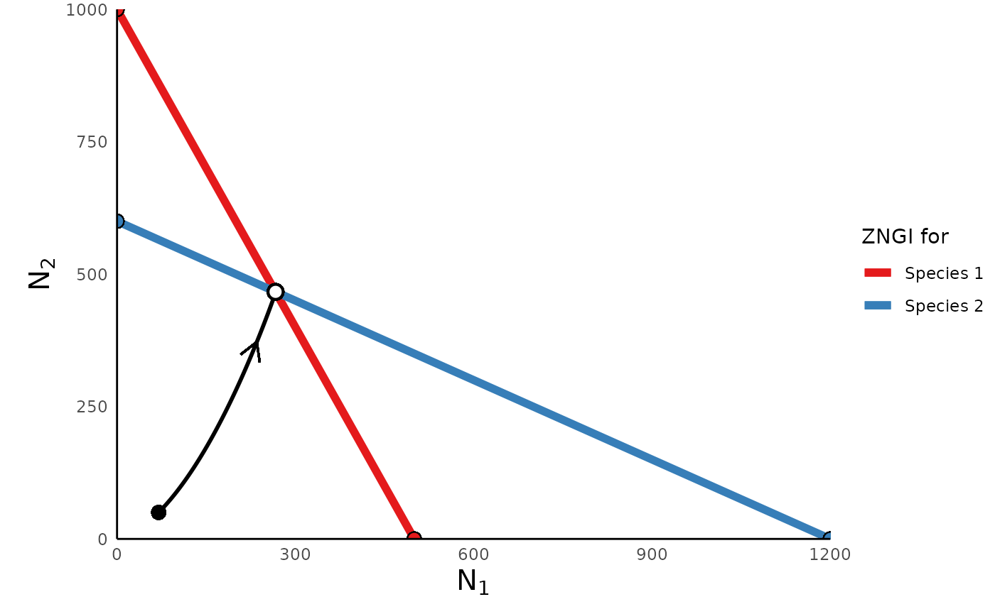
We can also plot the phase portrait of this model, which shows how N1
and N2 change relative to each other over time, using the function
plot_lvcomp_portrait(). In this case, we need to provide
the function the simulation generated above, as well as the parameter
vector we used to generate the simulation. The function uses this
information to plot the trajectory of the populations, as well as the
“zero net growth isoclines” (ZNGIs). (For more info about ZNGIs, please
refer to these resources: link 1, link
2):
plot_lvcomp_portrait(sim_df = lvcomp_simulation, params = lvcomp_params)
Lotka-Volterra competition in terms of absolute competition coefficients
In the equations above, we expressed the competitive effects of each species on itself (intraspecific competition) in terms of each species’ carrying capacity (\(K_1\) and \(K_2\)), and we described the species’ competitive effects on each other (interspecific competition) in terms of relative competition coefficients (\(\alpha\) and \(\beta\)). We can instead write the Lotka-Volterra competition equation in terms of the absolute effect of intra- and inter-specific competition on each species. Note that in these equations \(\alpha_{ii}\) represents the intraspecific competitive effect in species \(i\), and \(\alpha_{ij}\) describes the effect of species \(j\) on the growth of species \(i\):
\[\frac{dN_1}{dt} = r_1N_1(1-\alpha_{11}N_1 - \alpha_{12}N_2)\] \[\frac{dN_2}{dt} = r_2N_2(1-\alpha_{22}N_2 - \alpha_{21}N_1)\] Note that in this formulation, the carrying capacity of species 1 is simply the inverse of its intraspecific competition coefficient (\(K_1 = 1/{\alpha_{11}}\)), and similarly for species 2 (\(K_2 = 1/{\alpha_{22}}\)).
The run_lvcomp_model() function allows one to define the
parameters of Lotka-Volterra competition in this formulation, as shown
below:
lvcomp_params_abs <- c(r1 = .5, r2 = .5,
                       a11 = .002, a22 = .0016,
                       a12 = .0015, a21 = .001)
lvcomp_simulation_abs <- run_lvcomp_model(time = lvcomp_time, init = lvcomp_init,
                                          params = lvcomp_params_abs)

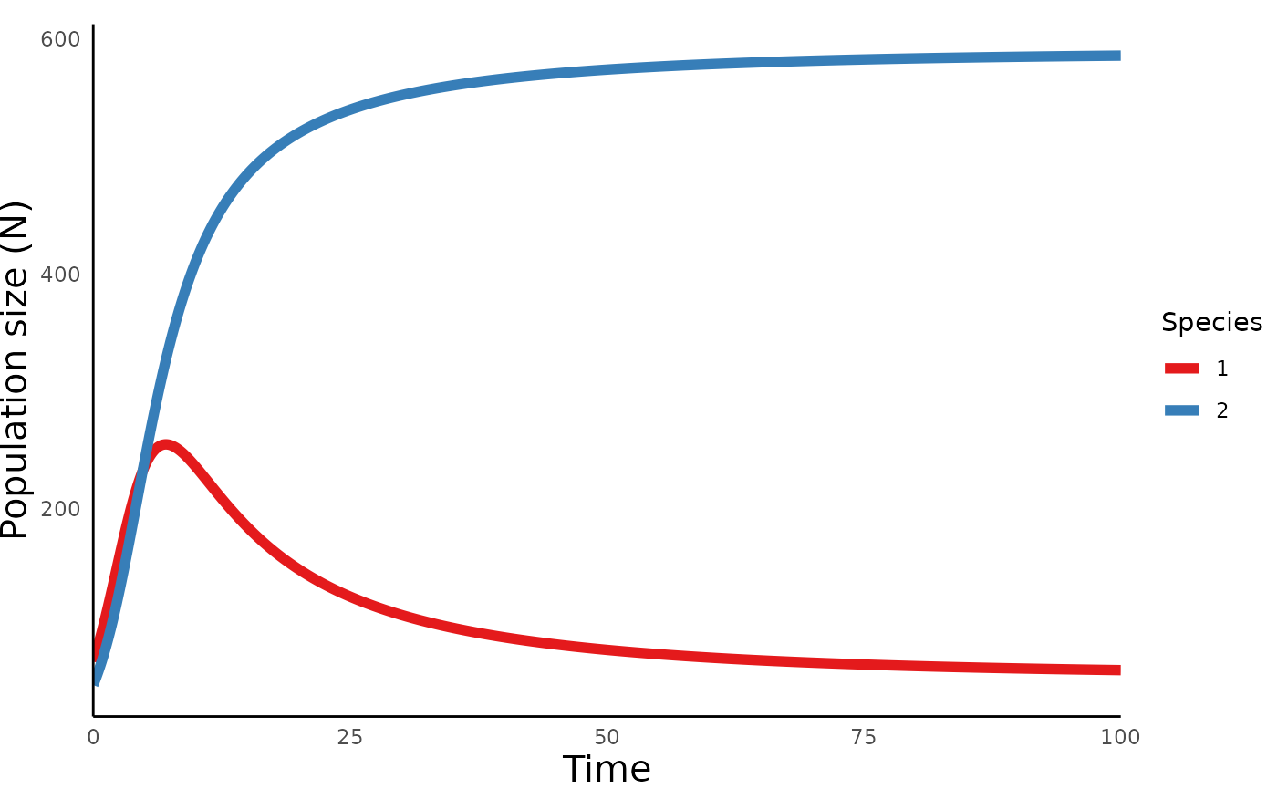
plot_lvcomp_time(lvcomp_simulation_abs)
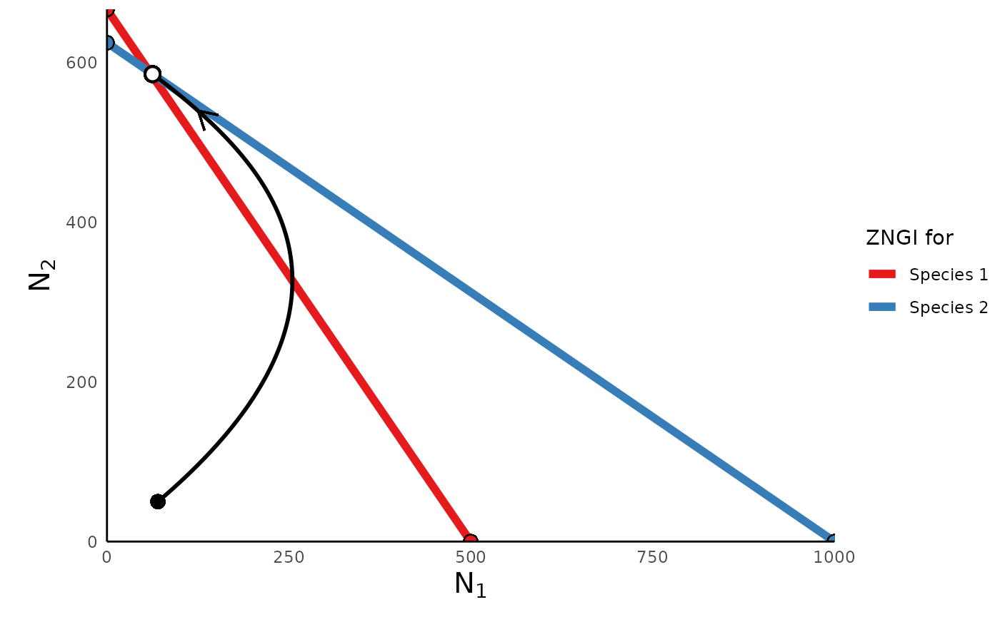
plot_lvcomp_portrait(lvcomp_simulation_abs, lvcomp_params_abs)
Other References
For more on the Lotka-Volterra competition model, please refer to the following references:
Dr. Hank Stevens’ chapter on Lotka-Volterra competition
Dr. Sarah Otto’s lecture notes on Lotka-Volterra competition.
Vandermeer and Goldberg, 2013. Population Ecology., Ch. 8. (Access to a digital copy of this textbook may be available through your library).
Rosenzweig and MacArthur, 1963. Graphical Representation and Stability Conditions of Predator-Prey Interactions. The American Naturalist. Note: this paper focuses on predator-prey models rather than species competition, but it presents a clear explanation of the concept of zero net-growth isoclines.