Island biogeography

library(ecoevoapps)
library(patchwork)

The theory of Island Biogeography, first articulated by Robert Macarthur and E.O. Wilson in the 1964 paper “Equilibrium theory of insular zoogeography”, presents a quantitative and predictive approach to understanding biodiversity on island systems. This framework assumes that species immigrate at higher rates from the mainland to nearby islands than to islands further away, and that extinction rates are higher in smaller islands than larger islands. The balance of these two processes determine an island’s equilibrium species richness. Macarthur and Wilson expanded on this theory in their classic 1967 book “The Theory of Island Biogeography”.

There are many ways to specifically turn this descriptive framework into a mathematical model – for example, we can model a linear relationship between island size and extinction rates, or we can imagine it as a nonlinear relationship. In this package we assume the following nonlinear relationships between island size and extinction rates, and between distance and immigration rates:

Extinction rate on island:

\[E = e^{\frac{kS}{A}}-1\]

Immigration rate from mainland to island: \[I = e^{\left(-\frac{k}{D}*(S-M)\right)}-1\]

This results in an equilibrium number of species on the island as follows:
\[S_{eq} = \frac{AM}{D+A}\]

where:

\(D\) is the distance from the mainland to the island (km);
\(A\) is the area of the island (km^2);
\(M\) is the number of species on the mainland;
\(k\) is the scaling constant (we set to \(k=0.015\) in this implementation, but the exact number is not very important).

We can simulate the dynamics of this model in R using the function run_ibiogeo_model(). This function runs the isoland biogeography model for two islands at a time, and we need to provide as inputs the size of the two islands and their distance from the mainland:

distances <- c(1, 2) # Distance of the two islands from mainland
areas <- c(2,2) # size (area) of the islands
ibiogeo_out <- run_ibiogeo_model(D = distances, A = areas)

The output from run_ibiogeo_model() is two plots – one of which is a diagram of a map showing the two islands, and the other which shows the immigration/extinction rates and resulting equilibrium species richness for the two islands:

ibiogeo_out$map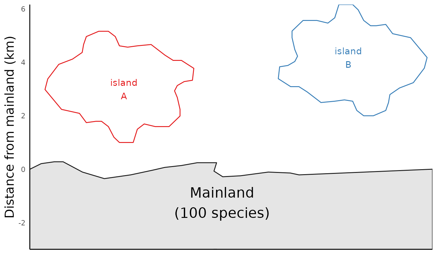

ibiogeo_out$eq_plot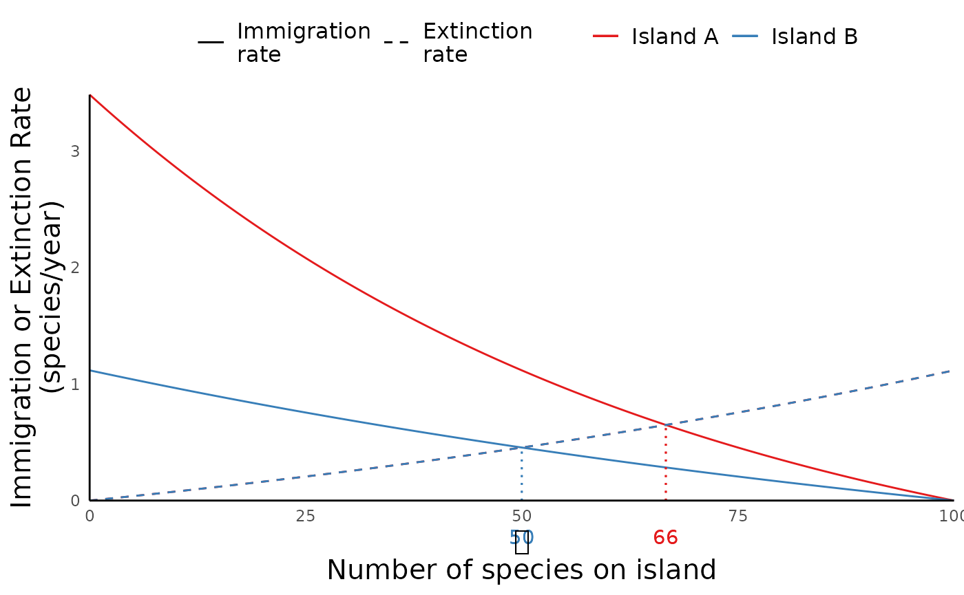

In this case, the extinction rate curve for both islands are same, since we set island sizes to be identical. This is why we just see the one line.

As we see in the map plots above, run_ibiogeo_model() assumes by default that the mainland is home to 100 species. But we can change this parameter as well:

mainland_richness <- 50
distances2 <- c(1, 2) # Distance of the two islands from mainland
areas2 <- c(2,1) # size (area) of the islands
ibiogeo_out2 <- run_ibiogeo_model(D = distances2, A = areas2, M = mainland_richness)

ibiogeo_out2$map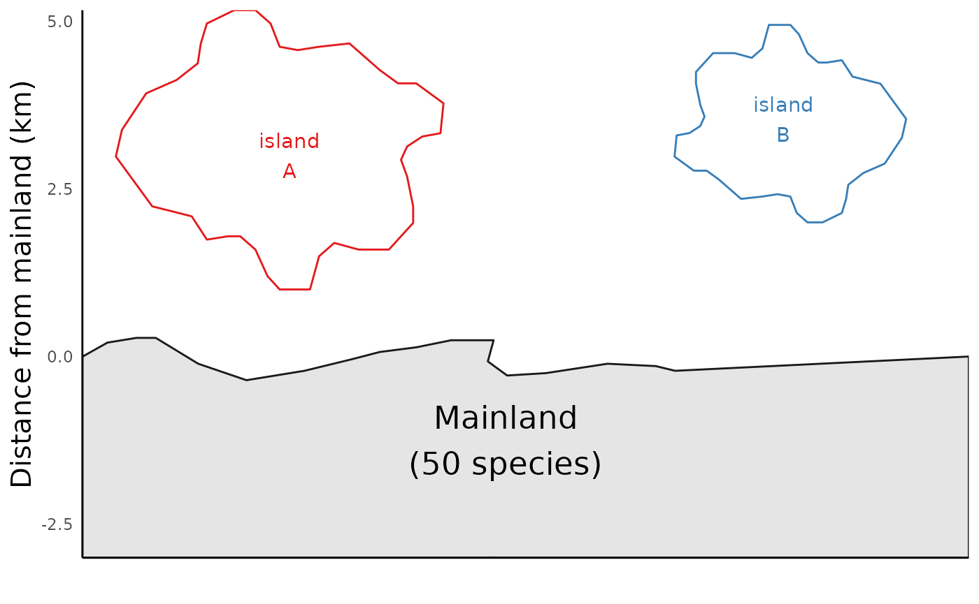


ibiogeo_out2$eq_plot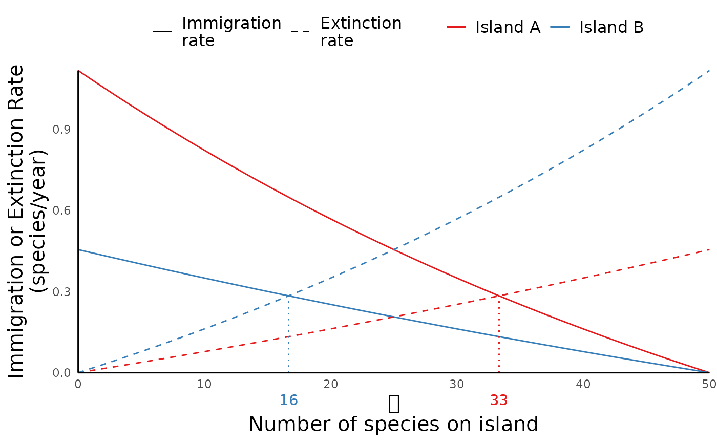

Further reading