Mutualisms • ecoevoapps

library(ecoevoapps)

Mutualism is a type of species interaction in which interacting species confer a net beneficial effect on one another. Mutualisms can manifest in various forms, including (but not limited to) plant-pollinator interactions, dispersal of seeds by animal vectors, and defense from predators. For example, fig wasps pollinate, lay eggs in, and feed on figs (Cook & Rasplus 2003). Another example is the mutualism between ants and acacia plants, in which ants feed on and shelter in acacias while protecting the plant from herbivores (Janzen 1966). A detailed overview of mutualisms can be found in Bronstein (2015).

The ecoevoapps package includes functions to simulate one specific mutualism model, which is described in more detail in Holland (2012). The core idea of the model is that each species’ population growth rate (\(dN/dt\)) is modified by interactions with both individuals of its own species and of another species, not unlike the classic Lotka-Volterra competition model. When it is growing alone, each species experiences intraspecific competition and grows in population size up to its population carrying capacity. But when the two species interact, they confer a benefit to each other, such that each species can grow to a population size beyond its carrying capacity. The model also assumes that there are diminishing returns on the beneficial effects of the mutualism, i.e. that the positive effects of each species level off at some population size.

Given these considerations, the model can be expressed as:

\[\frac{dN_1}{dt} = r_1N_1 + \frac{\alpha_{12}N_2}{b_2 + N_2}N_1 - d_1N_1^2\] \[\frac{dN_2}{dt} = r_2N_2 + \frac{\alpha_{21}N_1}{b_1 + N_1}N_2 - d_2N_2^2\]

This model can be simulated with the run_mutualism() function:

timevec <- seq(0, 10, by = 0.1)
start <- c(N1 = 100, N2 = 50)
pars <- c(r1 = 1, r2 = 1, a12 = 1.2, a21 = 0.8, b1 = 20, b2 = 20, d1 = 0.04, d2 = 0.02)
mut_out <- run_mutualism(time = timevec, init = start, params = pars)

head(mut_out)
#>   time        N1       N2
#> 1  0.0 100.00000 50.00000
#> 2  0.1  83.70023 53.21507
#> 3  0.2  73.81523 56.18362
#> 4  0.3  67.30379 58.89673
#> 5  0.4  62.77894 61.35311
#> 6  0.5  59.51722 63.55802

We can then use plot_mutualism_time() to plot the trajectory of these compartments over time:

plot_mutualism_time(mut_out)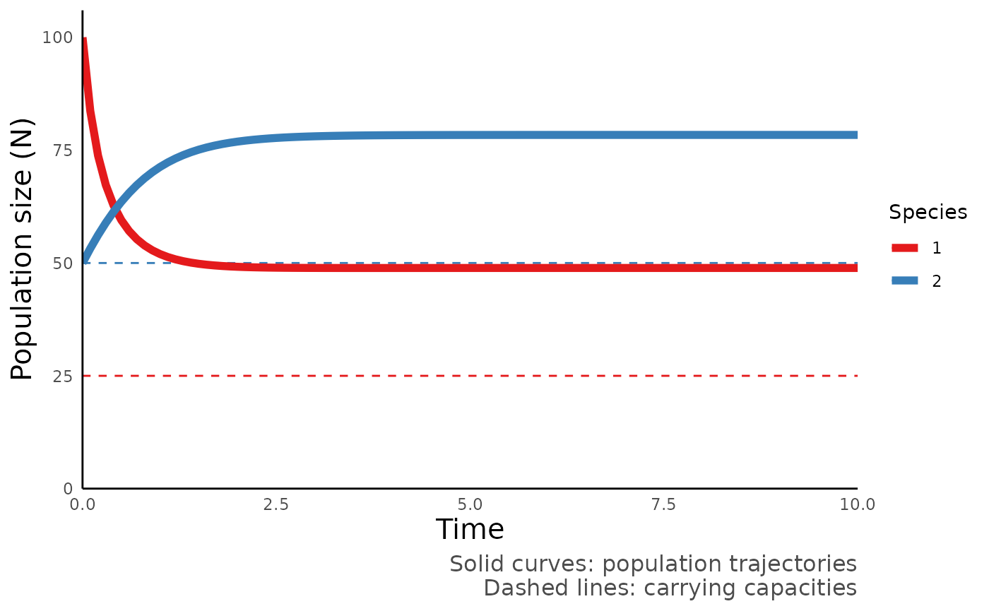

We can also plot the phase portrait of this model using the function plot_mutualism_portrait():

plot_mutualism_portrait(mut_out)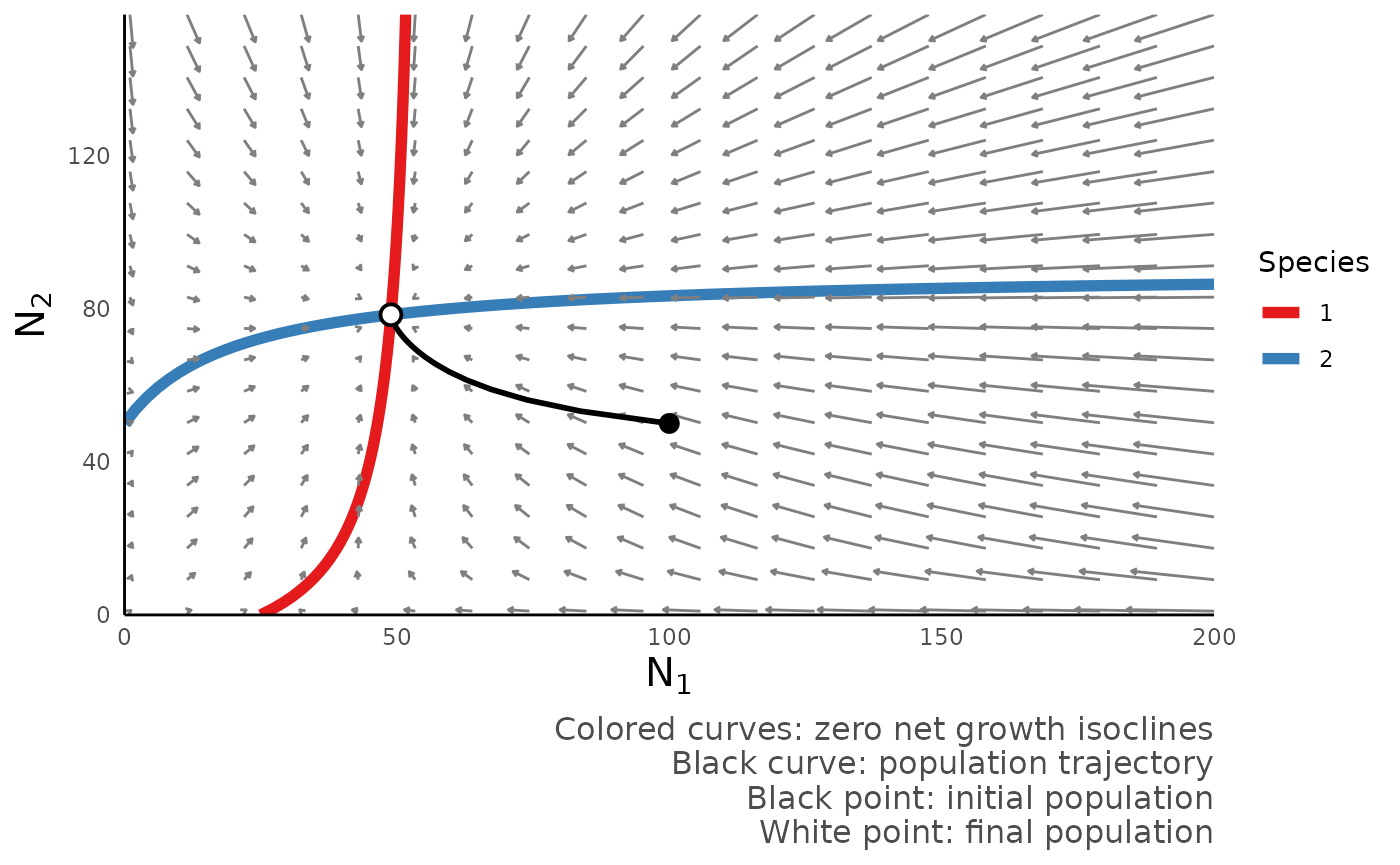

# To turn off the vector field, set vec = FALSE
# To turn off the realized trajectory, set traj = FALSE