Predator-prey interactions
predator-prey-interactions.RmdSome of the most dramatic species interactions in ecological communities are the interactions between predators and their prey. There is a long history in ecology of using mathematical equations to model the dynamics of this interaction. There are many versions of predator-prey dynamics models, but most share a few common features.
The prey species are considered as a single population which, in the absence of the predator, grows either exponentially or logistically. The predator, in turn, depends solely on the prey for its energy (i.e. it is a specialist predator), and if there were no prey available in the system, the predator population simply declines to zero. The more abundant the prey, the more the predator population can grow. But the more the predator population grows, the lower the prey falls. This sets up the cylic dynamics that we see in many predator-prey models.
We start this vignette with the Lotka-Volterra predator-prey model, and then build on this model by adding various levels of biological detail. In all models, \(H\) referes to the density of the prey, and \(P\) refers to the density of the predator. For a more detailed overview of the predator-prey models presented here, please refer to Dr. Hank Stevens’ Primer of Ecology using R.
Lotka-Volterra predator-prey dynamics
The classic Lotka-Volterra predator-prey model captures the dynamics between a prey species that has exponential growth, and a predator that consumes prey with no saturation point (in other words, there is a linear relationship between prey density and amount of prey consumer; refer to references on the functional response of predators for more details). This results in the following pair of equations:
\[ \frac{dH}{dt} = rH - aHP \\ \frac{dP}{dt} = eaHP - dP \] In the prey dynamics equation (\(dH/dt\)), the parameter \(r\) refers to the intrinsic per-capita growth rate of the prey; \(a\) refers to the attack rate of the predator, and \(H\) and \(P\) are the density of prey and predator respectively.
In the predator dynamics equation (\(dP/dt\)), \(e\) refers to the conversion efficiency, which is the rate at which the predator species can convert its food into new predator births. \(d\) refers to the intrinsic per-capita mortality rate of the predator.
We can simulate these dynamics with the ecoevoapps
functions run_predprey_model(), as follows:
time_lvpp <- seq(0,100, 0.1) # the time steps over which to run the simulation
params_lvpp <- c(r = .7, a = 0.1,  e = 0.2, d = .25)
init_lvpp <- c(H = 10, P = 10)
sim_df_lvpp <- run_predprey_model(time = time_lvpp, init = init_lvpp, params = params_lvpp)


head(sim_df_lvpp)
#>      time         H         P
#> [1,]  0.0 10.000000 10.000000
#> [2,]  0.1  9.706969  9.947194
#> [3,]  0.2  9.427761  9.889000
#> [4,]  0.3  9.162149  9.825787
#> [5,]  0.4  8.909858  9.757927
#> [6,]  0.5  8.670585  9.685775
plot_predprey_time(sim_df_lvpp)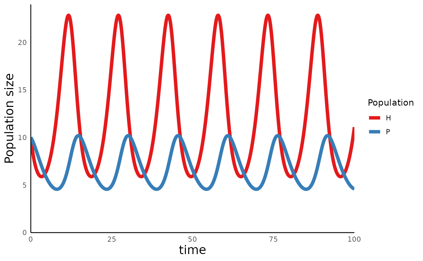
We can also plot the phase portrait of this model, which shows how N1
and N2 change relative to each other over time, using the function
plot_predprey_portrait(). In this case, we need to provide
the function the simulation generated above, as well as the parameter
vector we used to generate the simulation. The function uses this
information to plot the trajectory of the populations, as well as the
“zero net growth isoclines” (ZNGIs).1
plot_predprey_portrait(sim_df = sim_df_lvpp, params = params_lvpp)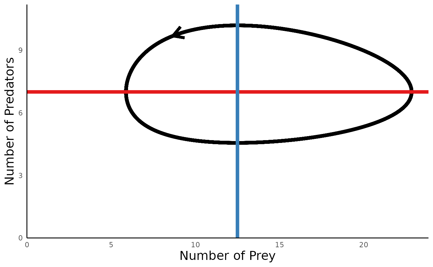 For predator-prey models, we can also add a layer under the actual
trajectory in the portrait diagrams, to show the vector field showing
how the population would move at all points in the phase space, using
the argument
 vectors_field = T:
plot_predprey_portrait(sim_df = sim_df_lvpp, params = params_lvpp, vectors_field = T)
#> Warning: Removed 221 rows containing missing values (geom_segment).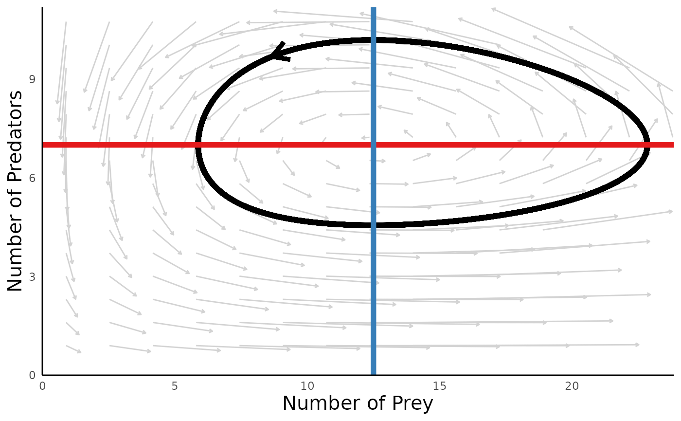
A key insight to emerge from this model is that these simple dynamics equations can give rise do cycles in the abundances of predators and preys, with no stationary equlibrium density to which the system settles.
Logistic growth in prey populations
In the classic Lotka-Volterra predator-prey model, the prey has exponential growth – the only check on prey population size is the consumption by the predator. One way useful layer of biological realism to the model is to introduce a carrying capacity for the prey population, as follows:
\[ \frac{dH}{dt} = rH \biggl(1-\frac{H}{K}\biggr) - aHP \\ \frac{dP}{dt} = eaHP - dP \]
In the prey dynamics equation (\(dH/dt\)), \(K\) represents the carrying capacity of the prey. The predator dynamics equation is unchanged from the model above.
We can again simulate this model with the function
run_predprey_model(), but now the parameter vector includes
an entry for the prey carrying capacity:
time_lvpp_K <- seq(0, 200, 0.1)
init_lvpp_K <- c(H = 15, P = 5)
# For the parameters vector, use the same entries in params_lvpp
# defined above, and add a carrying capacity of K = 500:
params_lvpp_K <- c(r = 1, K = 250, a = 0.1, e = 0.2, d = 0.25)
sim_df_lvpp_K <- run_predprey_model(time_lvpp_K, init_lvpp_K, params_lvpp_K)
head(sim_df_lvpp_K)
#>      time        H        P
#> [1,]  0.0 15.00000 5.000000
#> [2,]  0.1 15.67050 5.028419
#> [3,]  0.2 16.36129 5.063886
#> [4,]  0.3 17.07107 5.106751
#> [5,]  0.4 17.79820 5.157387
#> [6,]  0.5 18.54072 5.216187
We can again plot these dynamics using
plot_predprey_time() and
plot_predprey_portrait():
plot_predprey_time(sim_df_lvpp_K) +
  plot_predprey_portrait(sim_df_lvpp_K, params_lvpp_K)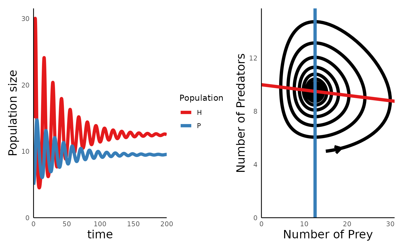
The plots above show us one of the key insights to emerge from this model: adding a carrying capacity to the prey adds a level of stabiity (self-regulation) to the system, such that over time, the cyclic dynamics between predator and prey give way to a stationary equilibrium point.
Type 2 function response in the predator
In the Lotka-Volterra model, the interaction between the predator and prey is set up such that the predator captures a fixed portion of the prey regardless of the prey’s abundance. This proportion is captured by the constant value \(a\) in the Lotka-Volterra equations. But in reality, there is likely some upper limit to the amount of prey that a predator can capture and process in a given amount of time. For example, some time may be spent in handling and/or digesting the prey – time during which the predator is not actively attacking yet more prey.
This upper limit to a predator’s consumption rates is captured by Type II functional response, and we can introduce this dynamic to the Lotka-Volterra equations as follows (note that in this formulation, the prey again has exponential growth):
\[ \frac{dH}{dt} = rH - \frac{aHP}{1+aT_hH} \\ \\ \frac{dP}{dt} = e \frac{aHP}{1+aT_hH} - dP \]
Here, the new variable \(T_h\) represents the “handling time” of the predator, and all other variables are as above.
One interesting outcome of introducing a handling time to the predator is that this destabilizes the system, such that the cyclic oscillations of predator and prey get larger in magnitude over time, which can increase the chance that one or both of the species crash to extinction. We can simulate these dynamics using the same functions:
# Parameters are as above; T_h is the handling time
params_tIIFR <- c(r = 0.5, a = 0.1, T_h = 0.2, e = 0.7, d = 0.3)
times_tIIFR <- seq(0, 50, 0.1)
init_tIIFR <- c(H = 10, P = 10)
sim_df_tIIFR <- run_predprey_model(time = times_tIIFR, init = init_tIIFR, params = params_tIIFR)
head(sim_df_tIIFR)
#>      time         H        P
#> [1,]  0.0 10.000000 10.00000
#> [2,]  0.1  9.658552 10.27888
#> [3,]  0.2  9.302664 10.54744
#> [4,]  0.3  8.935241 10.80353
#> [5,]  0.4  8.559266 11.04512
#> [6,]  0.5  8.177784 11.27030
Plotting the trajectory and portrait of these dynamics reveals the destabilizing effects of the functional response:
plot_predprey_time(sim_df_tIIFR) +
  plot_predprey_portrait(sim_df_tIIFR, params_tIIFR)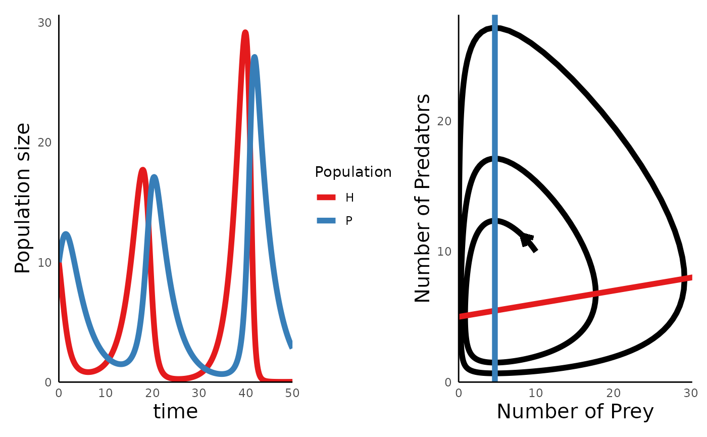
Logistic growth and Type II functional responses
In the previous two sections, we separately considered models of predator-prey dynamics with logistic growth in the prey or a predator with a type II functional response. We can put these features together into a single model, as follows:
\[ \frac{dH}{dt} = rH \biggl(1-\frac{H}{K}\biggr) - \frac{aHP}{1+aT_hH} \\ \\ \frac{dP}{dt} = e \frac{aHP}{1+aT_hH} - dP \]
In a series of papers in the 1960s and early 1970s, Robert Macarthur and Michael Rosenzweig analyzed the properties of this model, resulting in a classic 1971 paper by Rosenzweig describing the so-called “(paradox of enrichment)[https://en.wikipedia.org/wiki/Paradox_of_enrichment]”. The key insight was that in these models, higher values of the prey carrying capacit \(K\) can actually result in the crash and of the system.
We can use run_predprey_model() to simulate two sets of
dynamics that illustrate this paradox:
params_MR_lowK <- c(r = 0.5, K = 150, a = .02, T_h = .3, e = .6, d = .4)
params_MR_hiK <- c(r = 0.5, K = 350, a = .02, T_h = .3, e = .6, d = .4)
time_MR <- seq(0,100,0.1)
init_MR <- c(H = 10, P = 10)
sim_df_MR_lowK <- run_predprey_model(time = time_MR, init = init_MR, params = params_MR_lowK)
sim_df_MR_hiK <- run_predprey_model(time = time_MR, init = init_MR, params = params_MR_hiK)
plot_predprey_time(sim_df_MR_lowK) +
plot_predprey_time(sim_df_MR_hiK)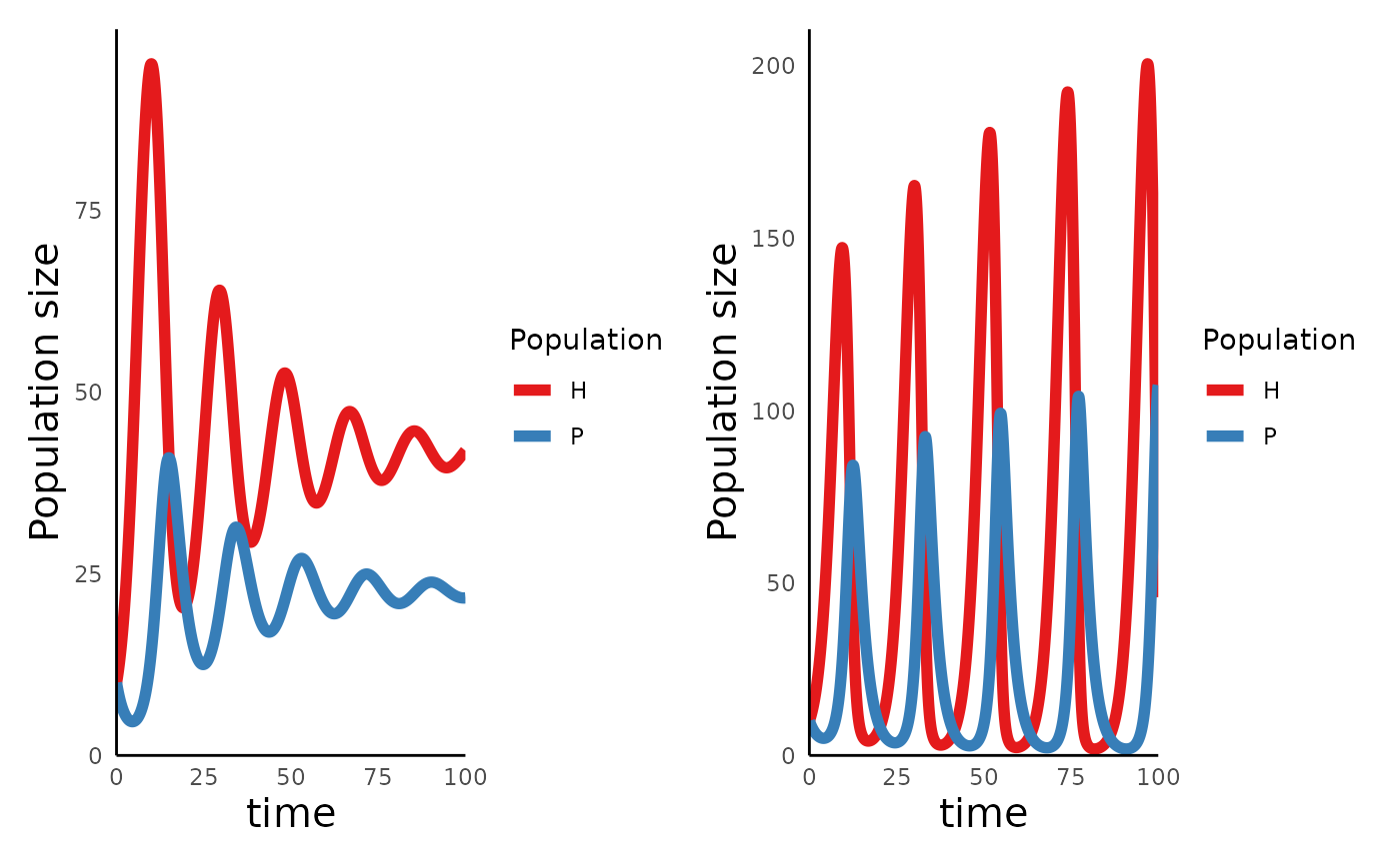 In the left hand plot, with \(K =
150\), the oscillations get smaller over time, and will
eventually reach a stationary equilibrium, while in the right, with
\(K = 350\), the magnitude of the
oscillations grows with time.
We can use plot_predprey_portrait() to evaluate why
these dynamics arise:
plot_predprey_portrait(sim_df_MR_lowK, params_MR_lowK) +
plot_predprey_portrait(sim_df_MR_hiK, params_MR_hiK) 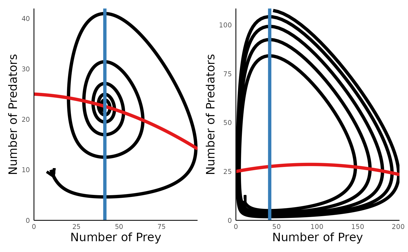
The key insight is that whether predator-prey dynamics lead to damped oscillations or oscillations that destabilize over time depends on the slope of the predator isocline when it intersects the prey isocline.
Other references
Consumer Resource Dynamics by Murdoch, Briggs and Nisbet - digital copy may be available through a library.
Graphical Representation and Stability Conditions of Predator-Prey Interactions, 1963, by M. L. Rosenzweig and R. H. MacArthur.
Some characteristics of simple types of predation and parasitism, 1959, by C.S. Holling.
Impact of Food and Predation on the Snowshoe Hare Cycle, 1995, by C.J. Krebs et al.
Dynamics of Predation, 2010, by A.N.P. Stevens
Additional references for Host-Parasite/Parasitoid
dynamics:
- Overivew
of the Nicholson-Bailey model (Links to Wikipedia page)
- Modelling
the biological control of insect pests: a review of host-parasitoid
models, 1996, by N.J. Mills and W.M. Getz